


On this article we’ll type an intensive understanding of the neural community, a cornerstone know-how underpinning nearly all innovative AI programs. We’ll first discover neurons within the human mind, after which discover how they fashioned the elemental inspiration for neural networks in AI. We’ll then discover back-propagation, the algorithm used to coach neural networks to do cool stuff. Lastly, after forging an intensive conceptual understanding, we’ll implement a Neural Community ourselves from scratch and prepare it to resolve a toy downside.
Who’s this convenient for? Anybody who needs to type a whole understanding of the cutting-edge of AI.
How superior is that this publish? This text is designed to be accessible to newcomers, and in addition incorporates thorough info which can function a helpful refresher for extra skilled readers.
Pre-requisites: None
Inspiration From the Mind
Neural networks take direct inspiration from the human mind, which is made up of billions of extremely complicated cells known as neurons.
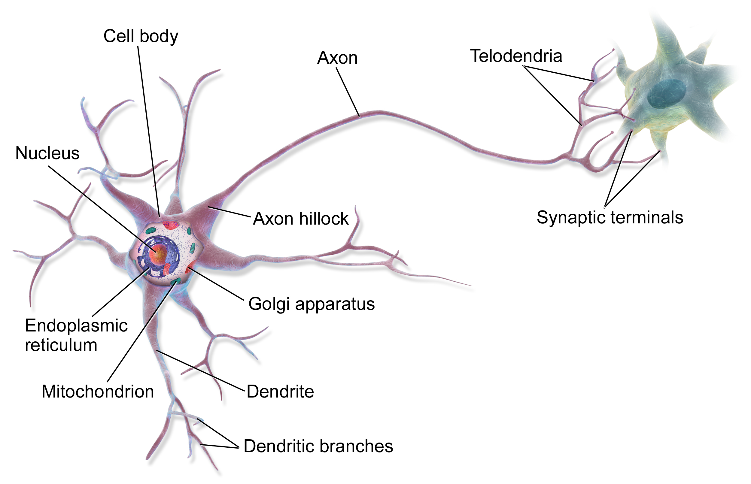
The method of considering inside the human mind is the results of communication between neurons. You would possibly obtain stimulus within the type of one thing you noticed, then that info is propagated to neurons within the mind by way of electrochemical indicators.

The primary neurons within the mind obtain that stimulus, then every neuron might select whether or not or to not “hearth” primarily based on how a lot stimulus it acquired. “Firing”, on this case, is a neurons choice to ship indicators to the neurons it’s linked to.

Then the neurons which these Neurons are linked to might or might not select to fireplace.
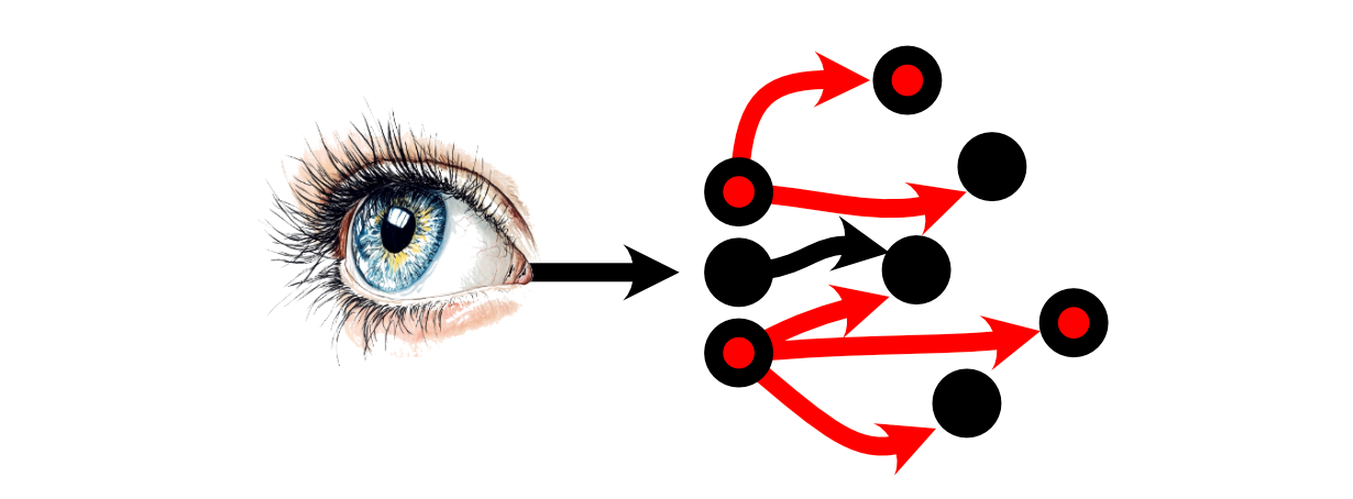
Thus, a “thought” will be conceptualized as numerous neurons selecting to, or to not hearth primarily based on the stimulus from different neurons.
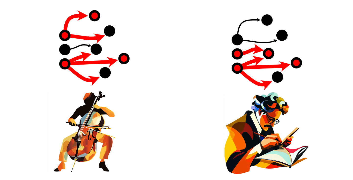
As one navigates all through the world, one might need sure ideas greater than one other individual. A cellist would possibly use some neurons greater than a mathematician, as an illustration.
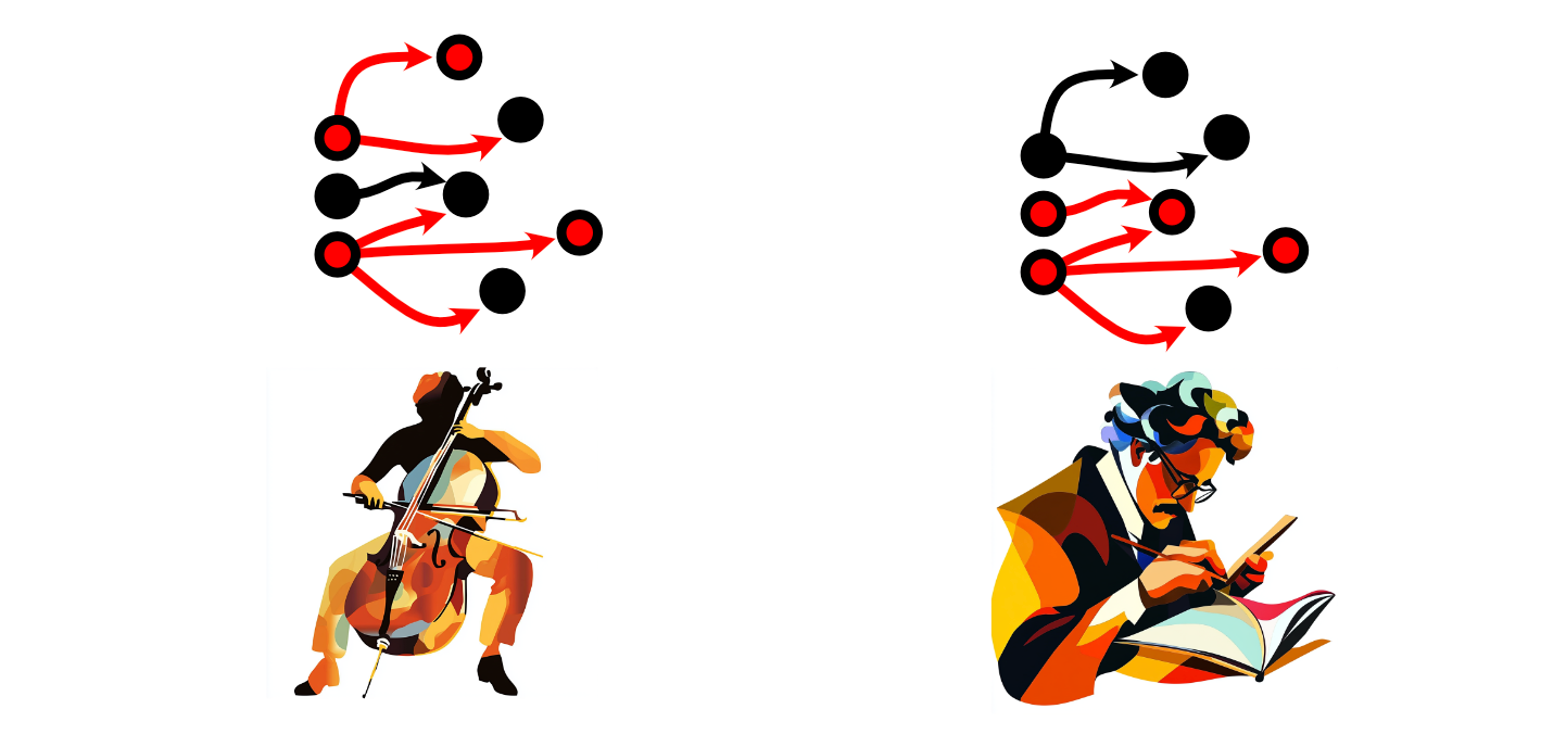
Once we use sure neurons extra continuously, their connections develop into stronger, growing the depth of these connections. Once we don’t use sure neurons, these connections weaken. This basic rule has impressed the phrase “Neurons that fireplace collectively, wire collectively”, and is the high-level high quality of the mind which is liable for the training course of.
I’m not a neurologist, so in fact this can be a tremendously simplified description of the mind. Nevertheless, it’s sufficient to know the elemental concept of a neural community.
The Instinct of Neural Networks
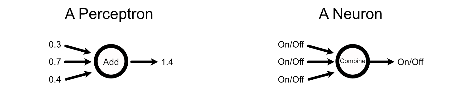
Neural networks are, primarily, a mathematically handy and simplified model of neurons inside the mind. A neural community is made up of components known as “perceptrons”, that are immediately impressed by neurons.
 1, source 2](https://towardsdatascience.com/wp-content/uploads/2025/02/1Vp3uVTyAcixfAlwcZWTTbQ.png)
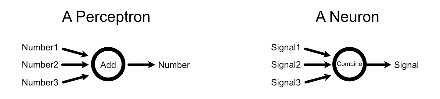
Perceptrons soak up knowledge, like a neuron does,
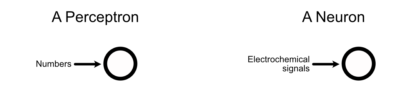
combination that knowledge, like a neuron does,
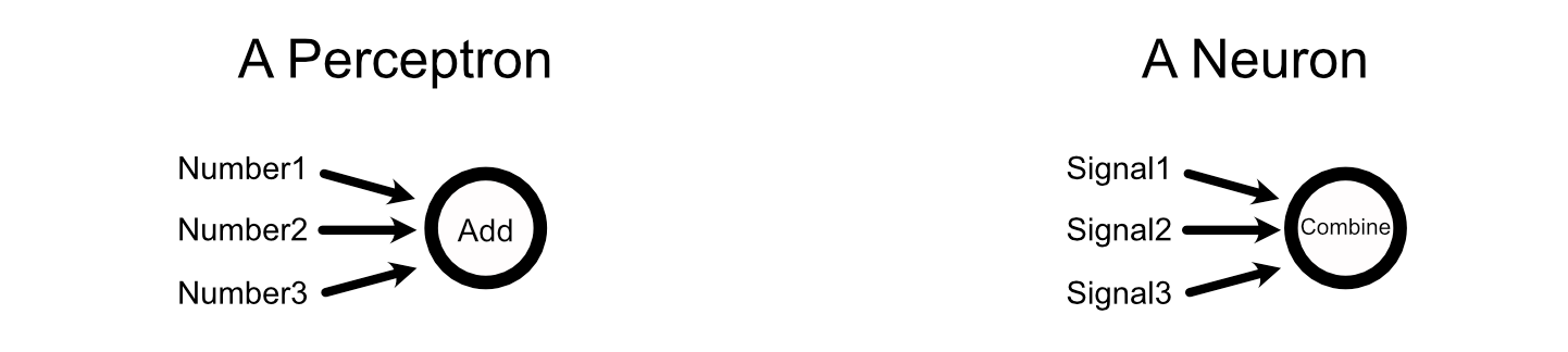
then output a sign primarily based on the enter, like a neuron does.
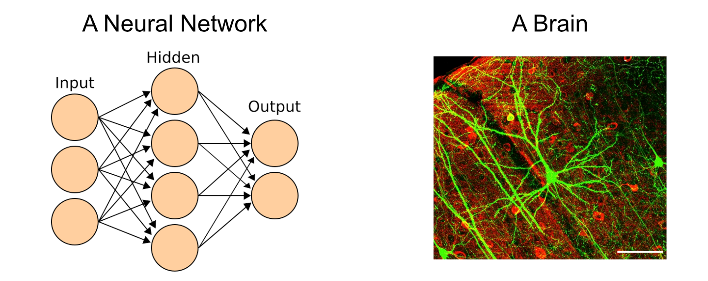
A neural community will be conceptualized as a giant community of those perceptrons, similar to the mind is a giant community of neurons.
When a neuron within the mind fires, it does in order a binary choice. Or, in different phrases, neurons both hearth or they don’t. Perceptrons, then again, don’t “hearth” per-se, however output a spread of numbers primarily based on the perceptrons enter.
Neurons inside the mind can get away with their comparatively easy binary inputs and outputs as a result of ideas exist over time. Neurons primarily pulse at completely different charges, with slower and quicker pulses speaking completely different info.
So, neurons have easy inputs and outputs within the type of on or off pulses, however the price at which they pulse can talk complicated info. Perceptrons solely see an enter as soon as per cross via the community, however their enter and output could be a steady vary of values. In the event you’re acquainted with electronics, you would possibly mirror on how that is much like the connection between digital and analogue indicators.
The way in which the maths for a perceptron truly shakes out is fairly easy. A normal neural community consists of a bunch of weights connecting the perceptron’s of various layers collectively.
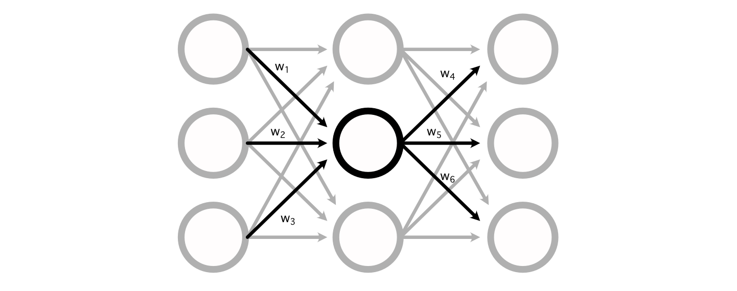
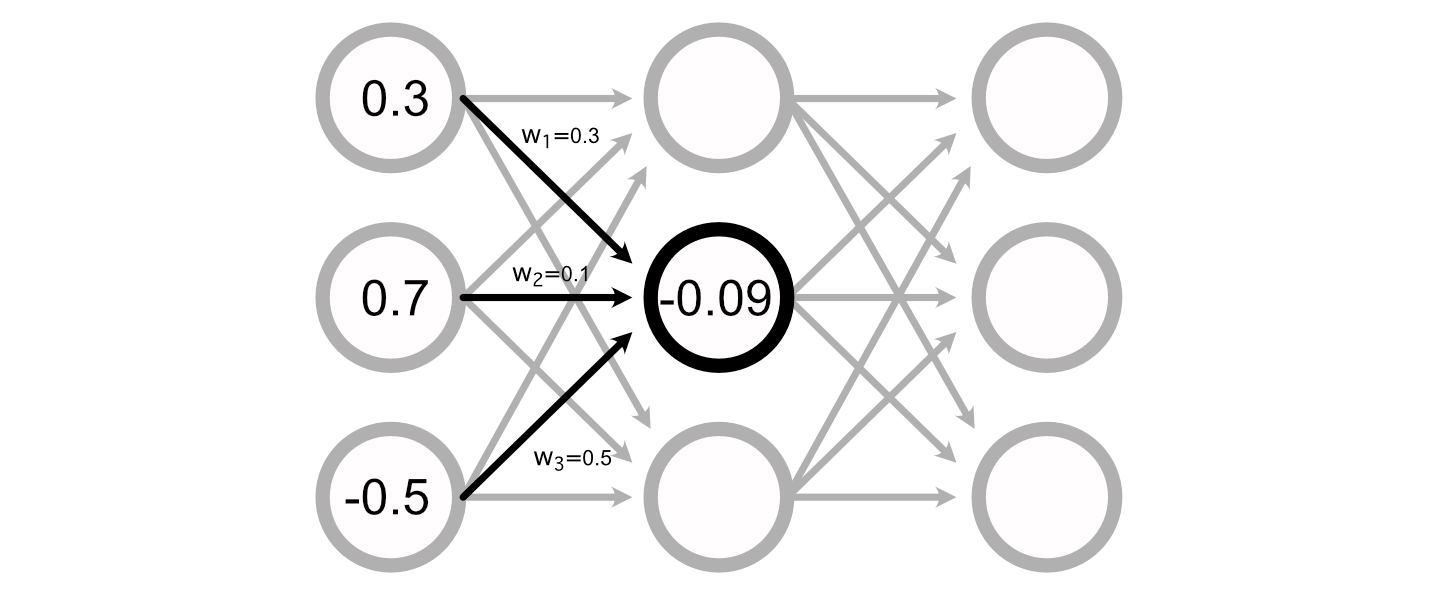
You’ll be able to calculate the worth of a selected perceptron by including up all of the inputs, multiplied by their respective weights.
Many Neural Networks even have a “bias” related to every perceptron, which is added to the sum of the inputs to calculate the perceptron’s worth.
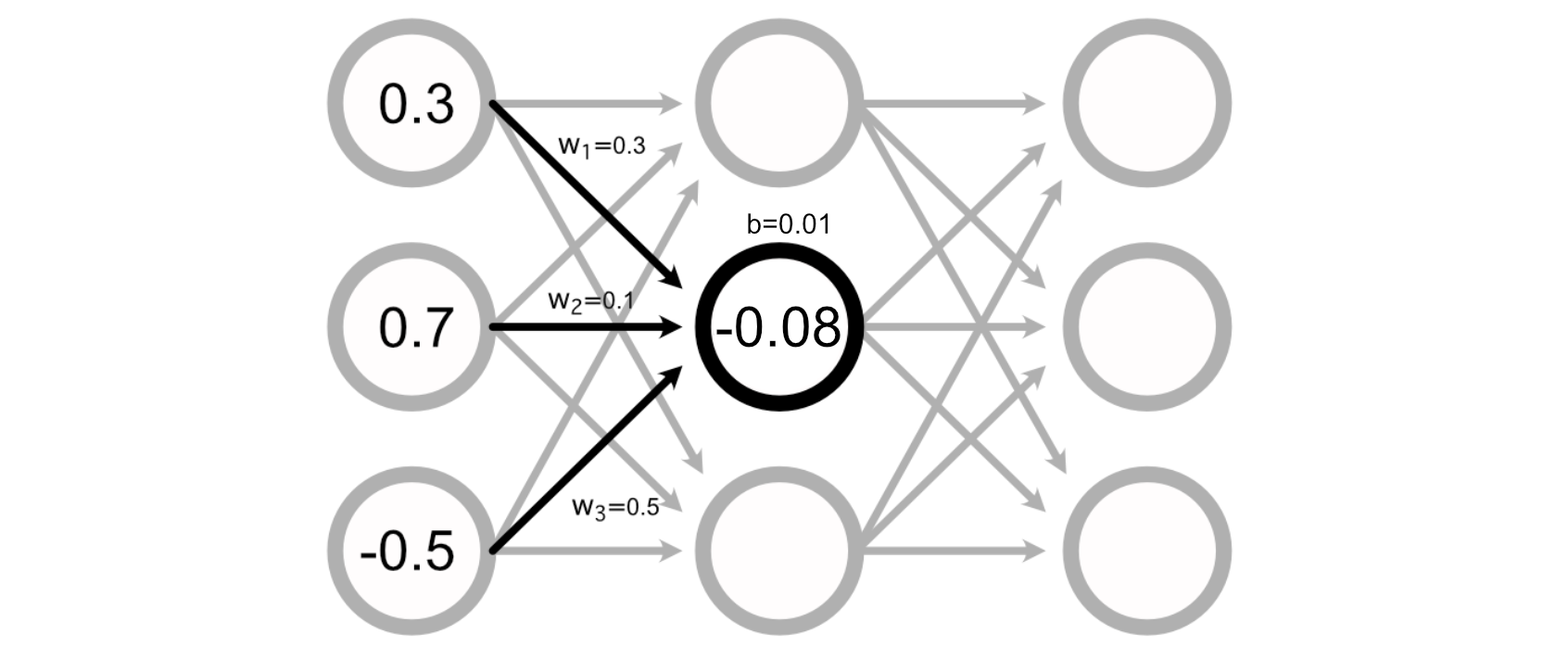
Calculating the output of a neural community, then, is simply doing a bunch of addition and multiplication to calculate the worth of all of the perceptrons.
Generally knowledge scientists confer with this basic operation as a “linear projection”, as a result of we’re mapping an enter into an output by way of linear operations (addition and multiplication). One downside with this strategy is, even in case you daisy chain a billion of those layers collectively, the ensuing mannequin will nonetheless simply be a linear relationship between the enter and output as a result of it’s all simply addition and multiplication.
This can be a major problem as a result of not all relationships between an enter and output are linear. To get round this, knowledge scientists make use of one thing known as an “activation operate”. These are non-linear features which will be injected all through the mannequin to, primarily, sprinkle in some non-linearity.
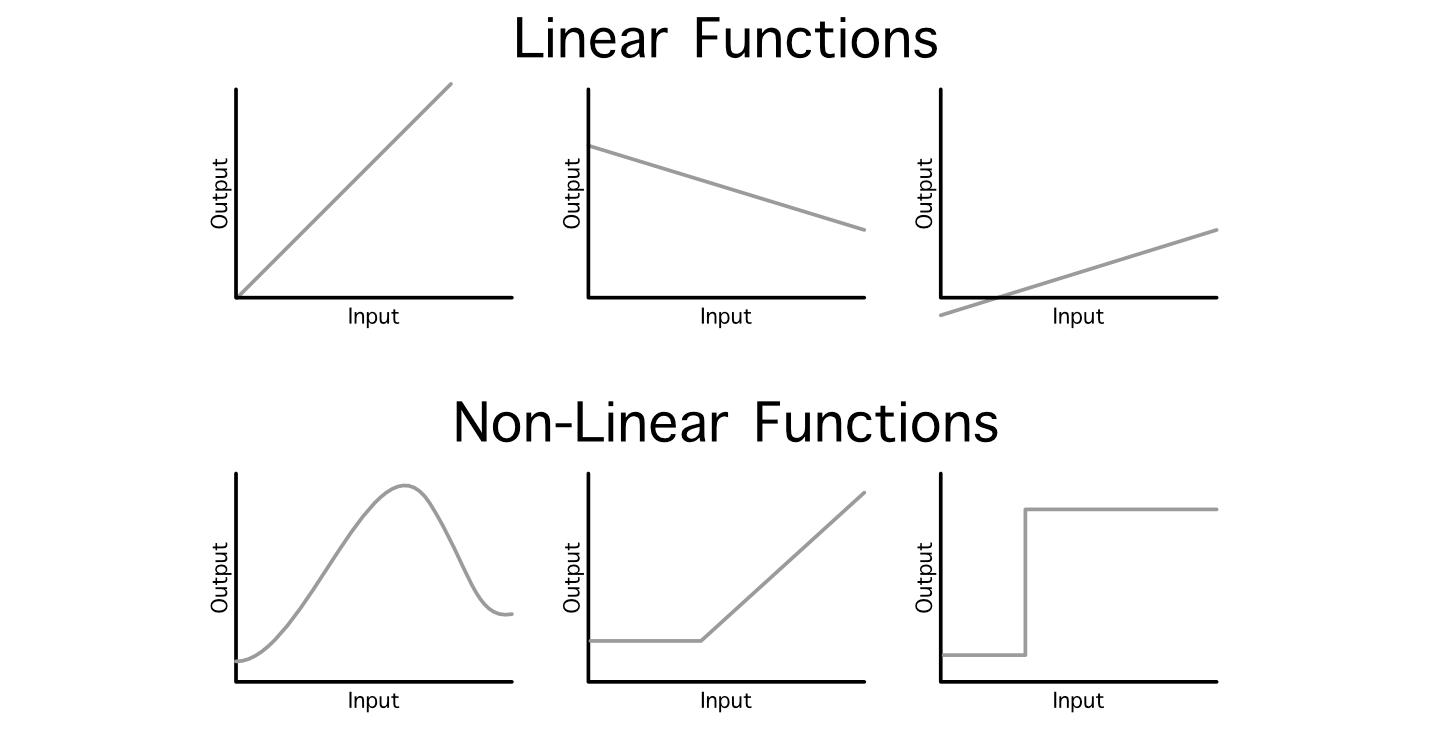
by interweaving non-linear activation features between linear projections, neural networks are able to studying very complicated features,
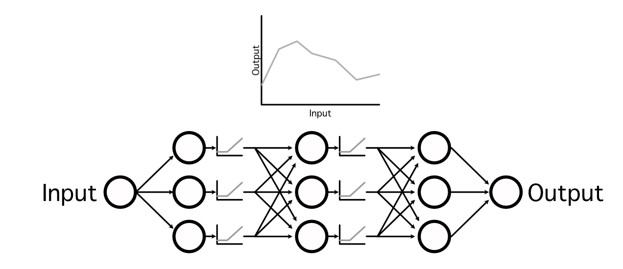
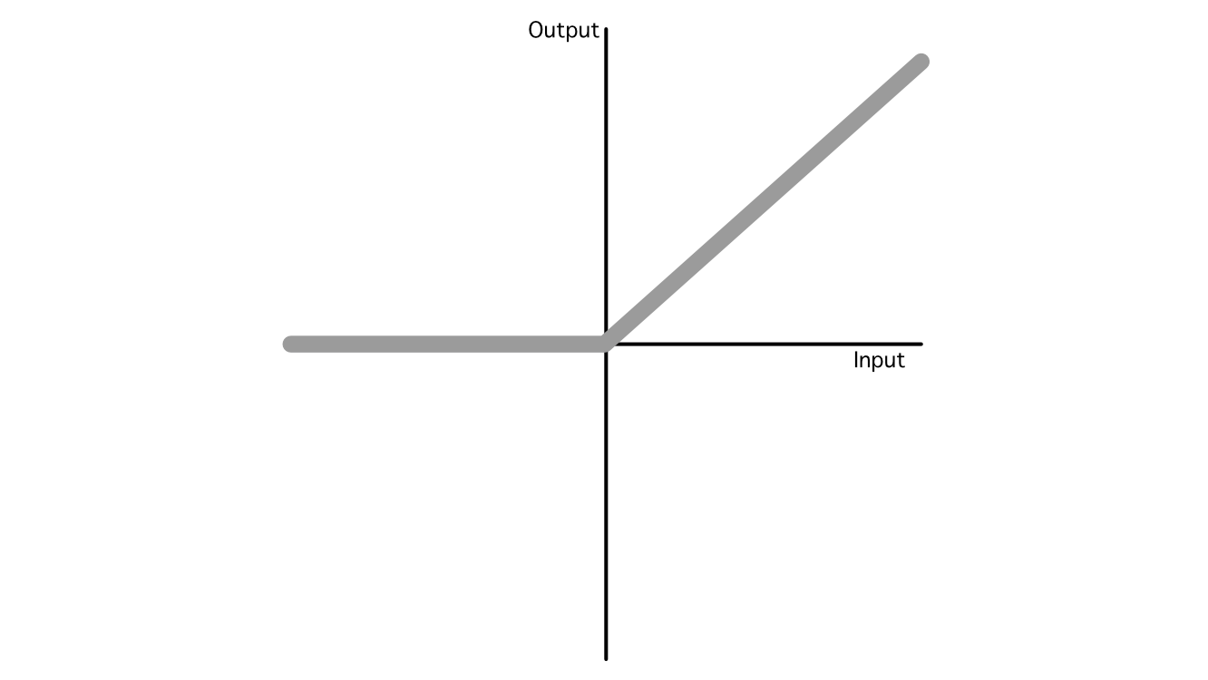
In AI there are numerous fashionable activation features, however the business has largely converged on three fashionable ones: ReLU, Sigmoid, and Softmax, that are utilized in quite a lot of completely different purposes. Out of all of them, ReLU is the most typical because of its simplicity and talent to generalize to imitate virtually some other operate.
So, that’s the essence of how AI fashions make predictions. It’s a bunch of addition and multiplication with some nonlinear features sprinkled in between.
One other defining attribute of neural networks is that they are often educated to be higher at fixing a sure downside, which we’ll discover within the subsequent part.
Again Propagation
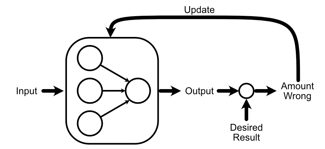
One of many basic concepts of AI is which you can “prepare” a mannequin. That is executed by asking a neural community (which begins its life as a giant pile of random knowledge) to do some activity. Then, you one way or the other replace the mannequin primarily based on how the mannequin’s output compares to a recognized good reply.
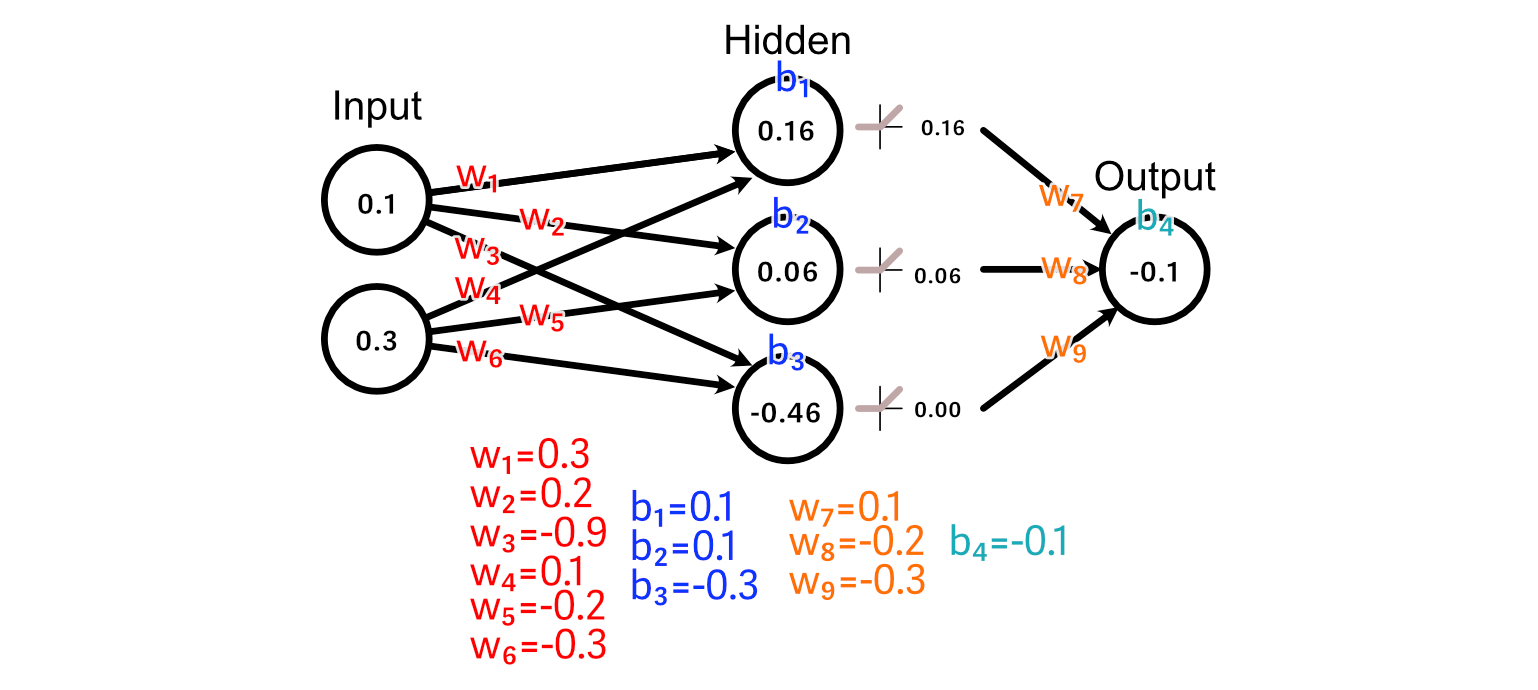
For this part, let’s think about a neural community with an enter layer, a hidden layer, and an output layer.
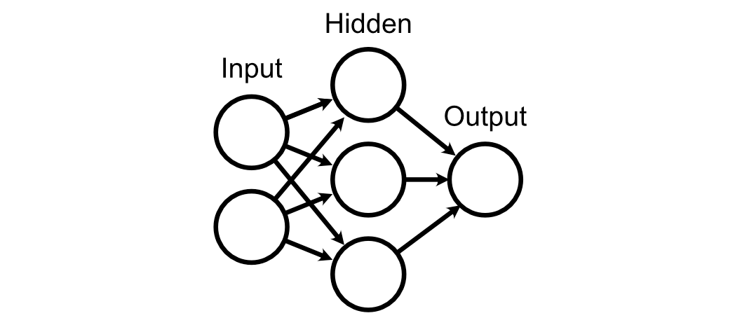
Every of those layers are linked along with, initially, utterly random weights.
And we’ll use a ReLU activation operate on our hidden layer.
Let’s say we now have some coaching knowledge, by which the specified output is the common worth of the enter.
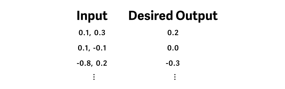
And we cross an instance of our coaching knowledge via the mannequin, producing a prediction.
To make our neural community higher on the activity of calculating the common of the enter, we first evaluate the expected output to what our desired output is.
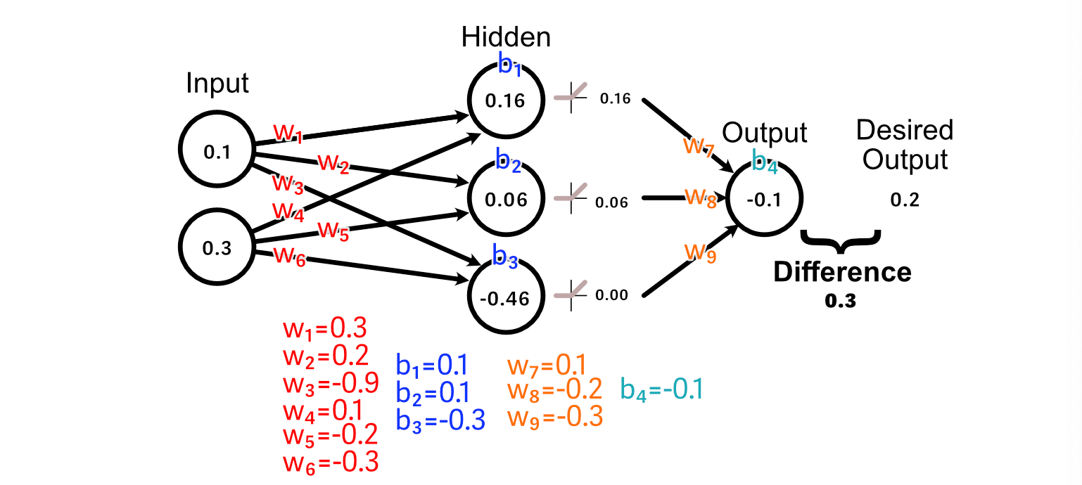
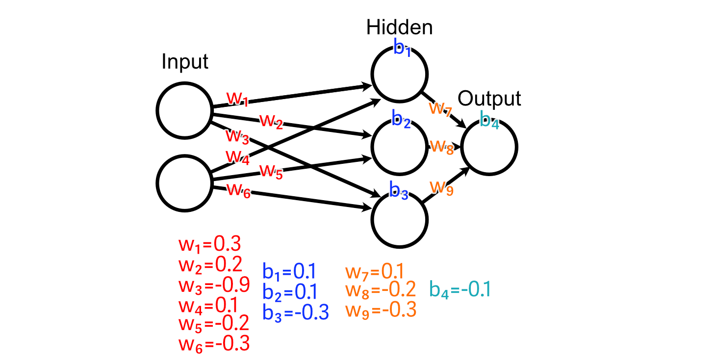
Now that we all know that the output ought to enhance in measurement, we are able to look again via the mannequin to calculate how our weights and biases would possibly change to advertise that change.
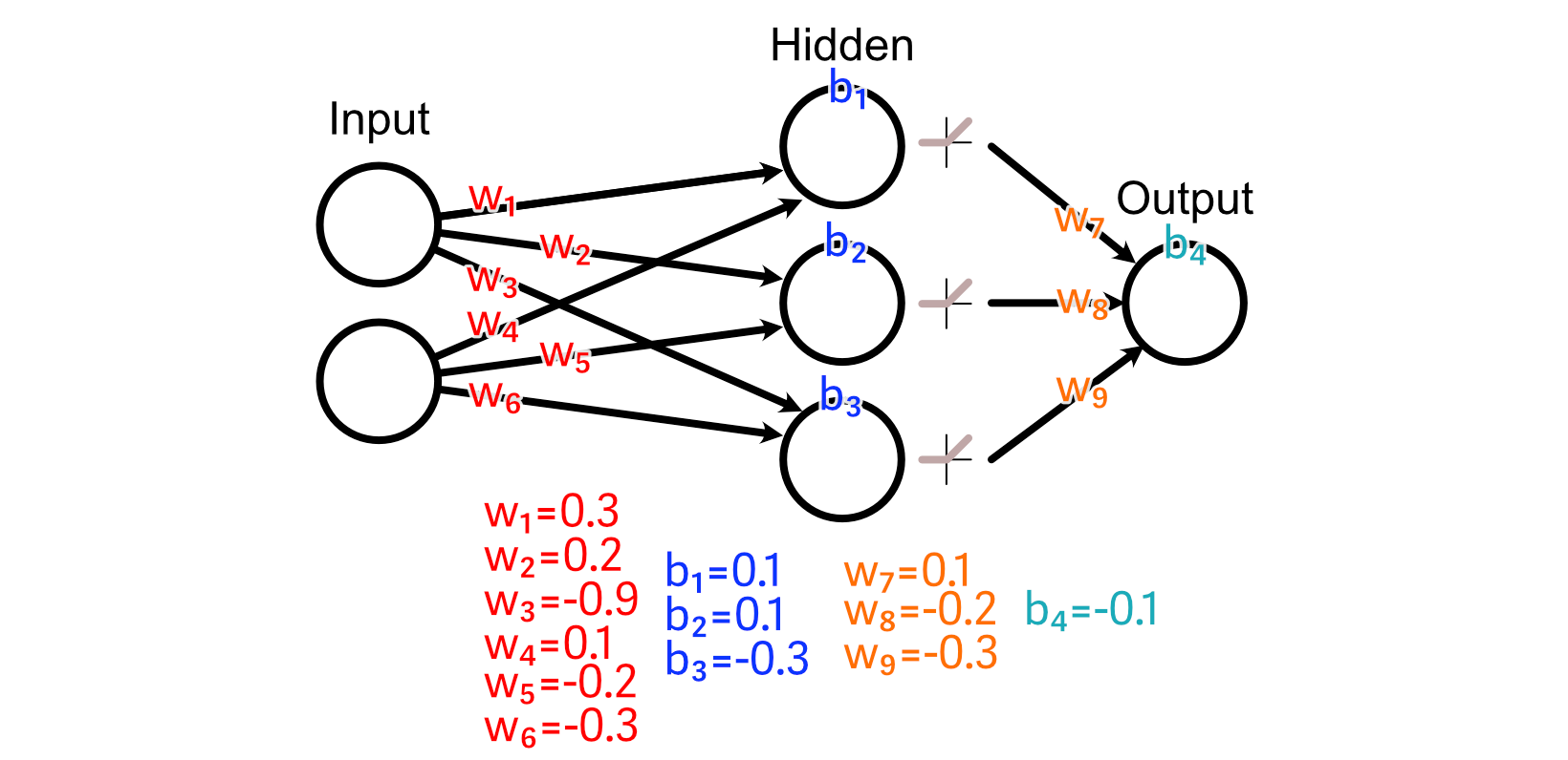
First, let’s take a look at the weights main instantly into the output: w₇, w₈, w₉. As a result of the output of the third hidden perceptron was -0.46, the activation from ReLU was 0.00.
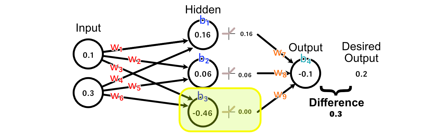
Consequently, there’s no change to w₉ that might consequence us getting nearer to our desired output, as a result of each worth of w₉ would lead to a change of zero on this explicit instance.
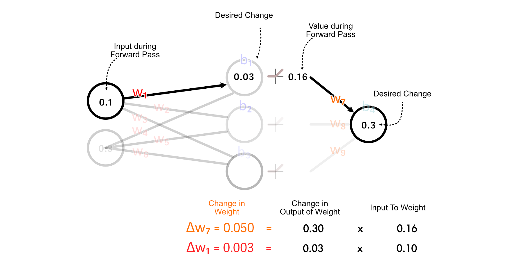
The second hidden neuron, nevertheless, does have an activated output which is larger than zero, and thus adjusting w₈ will have an effect on the output for this instance.

The way in which we truly calculate how a lot w₈ ought to change is by multiplying how a lot the output ought to change, occasions the enter to w₈.
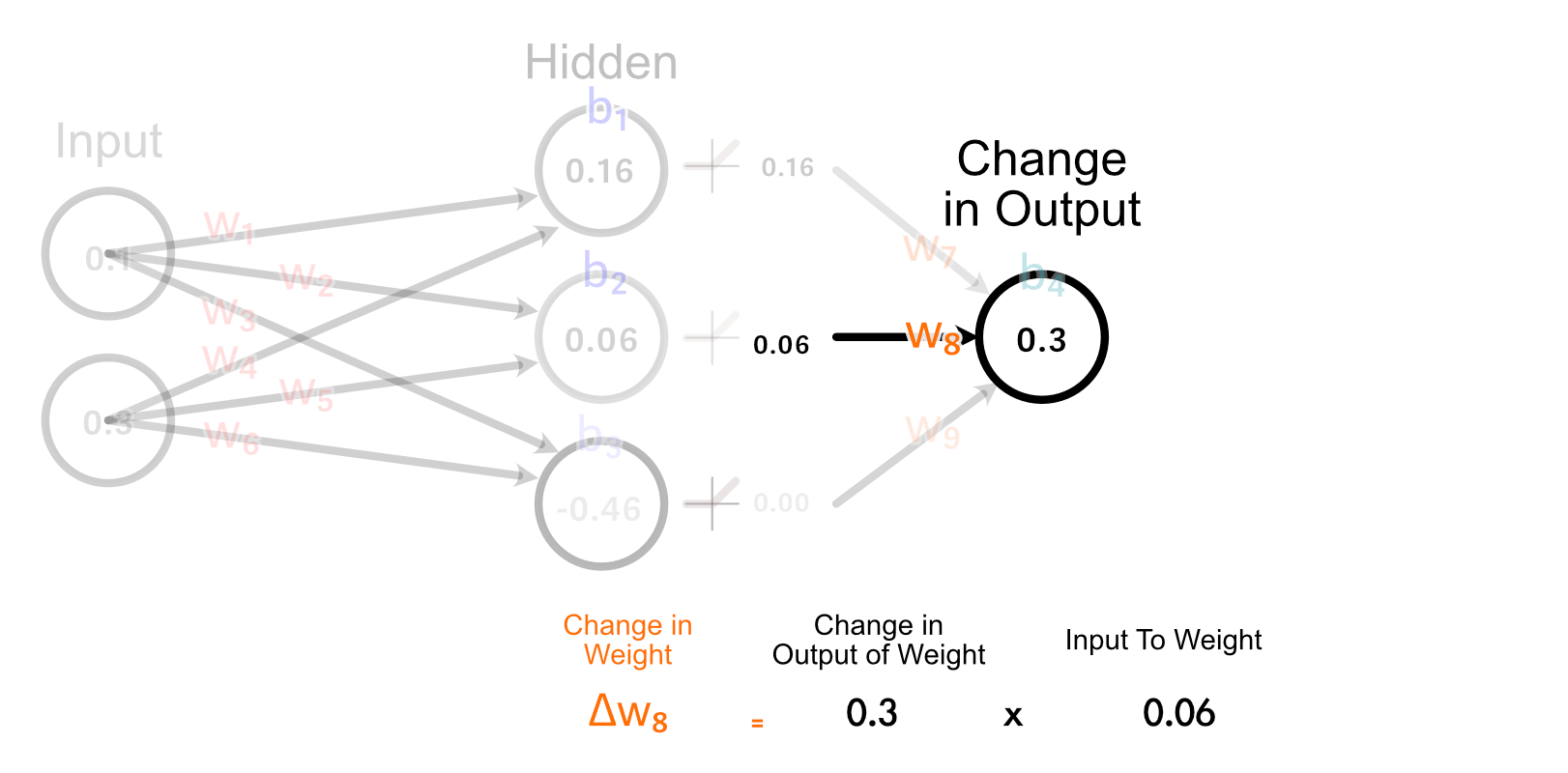
The simplest clarification of why we do it this fashion is “as a result of calculus”, but when we take a look at how all weights get up to date within the final layer, we are able to type a enjoyable instinct.
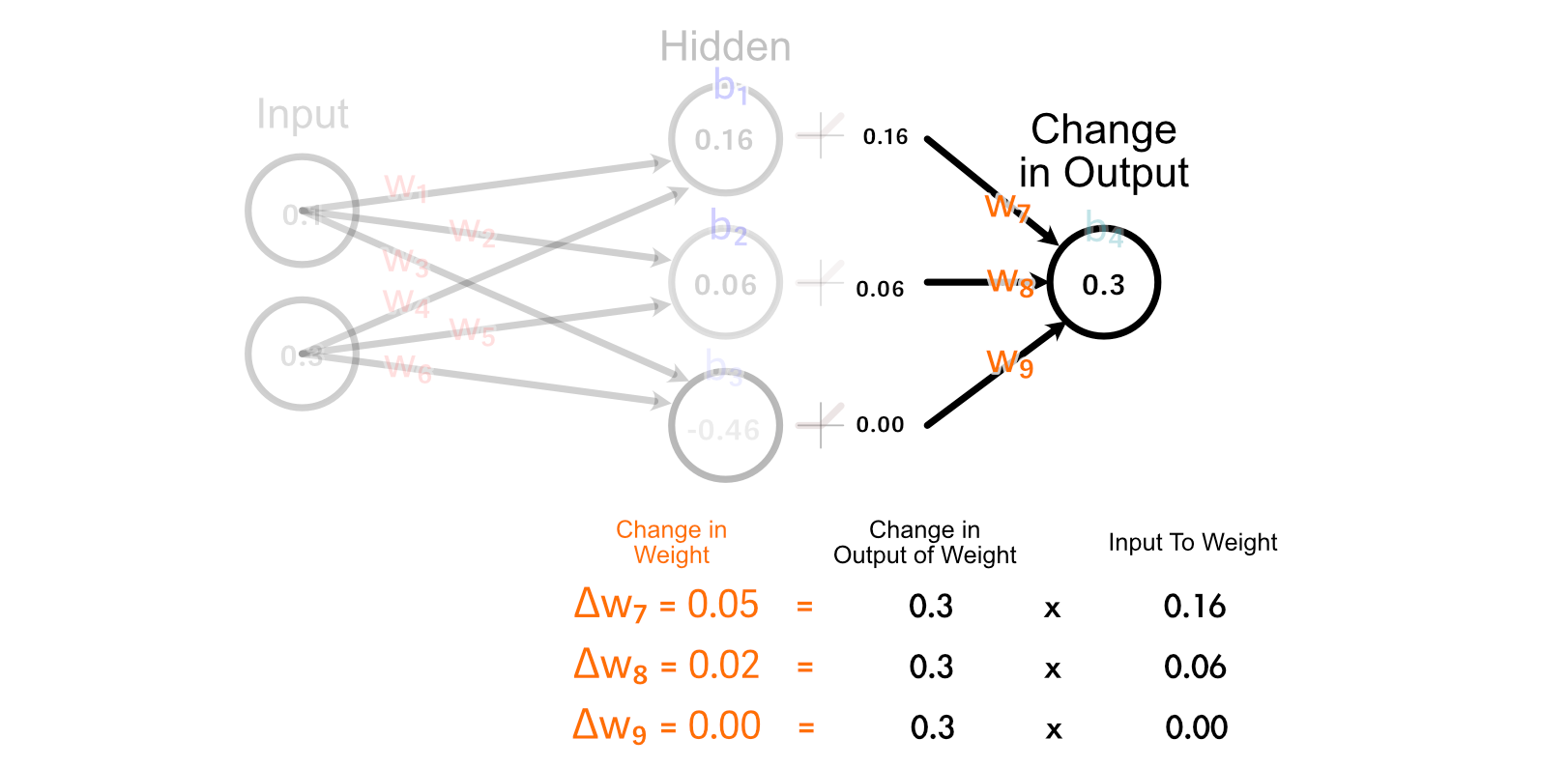
Discover how the 2 perceptrons that “hearth” (have an output larger than zero) are up to date collectively. Additionally, discover how the stronger a perceptrons output is, the extra its corresponding weight is up to date. That is considerably much like the concept that “Neurons that fireplace collectively, wire collectively” inside the human mind.
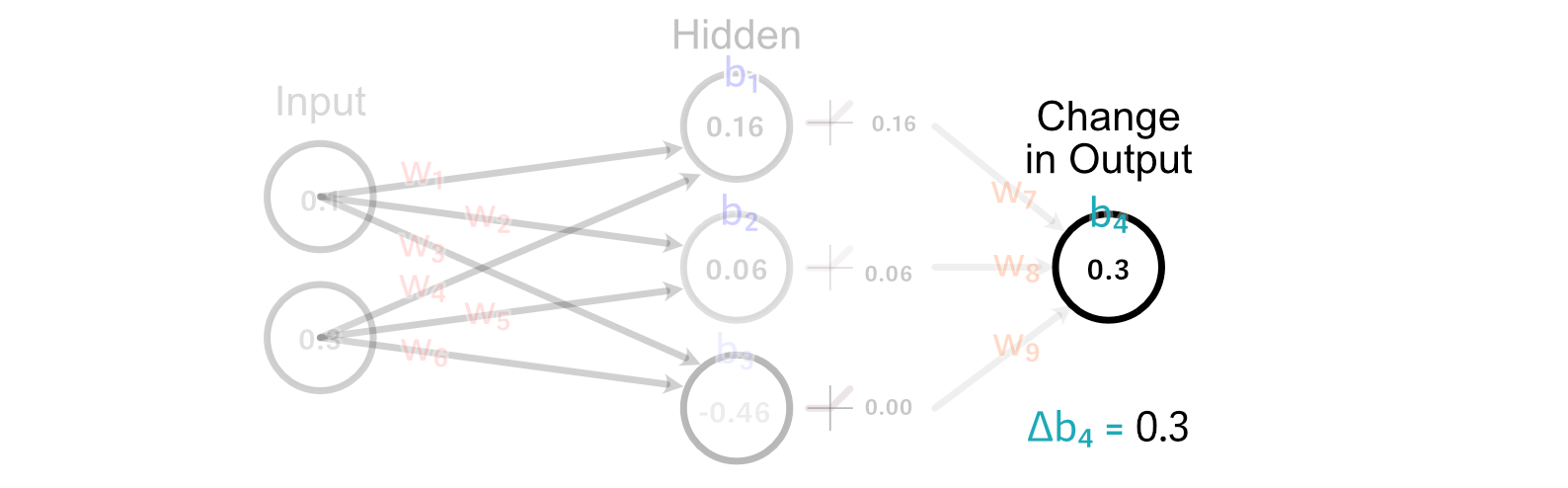
Calculating the change to the output bias is tremendous simple. In actual fact, we’ve already executed it. As a result of the bias is how a lot a perceptrons output ought to change, the change within the bias is simply the modified within the desired output. So, Δb₄=0.3
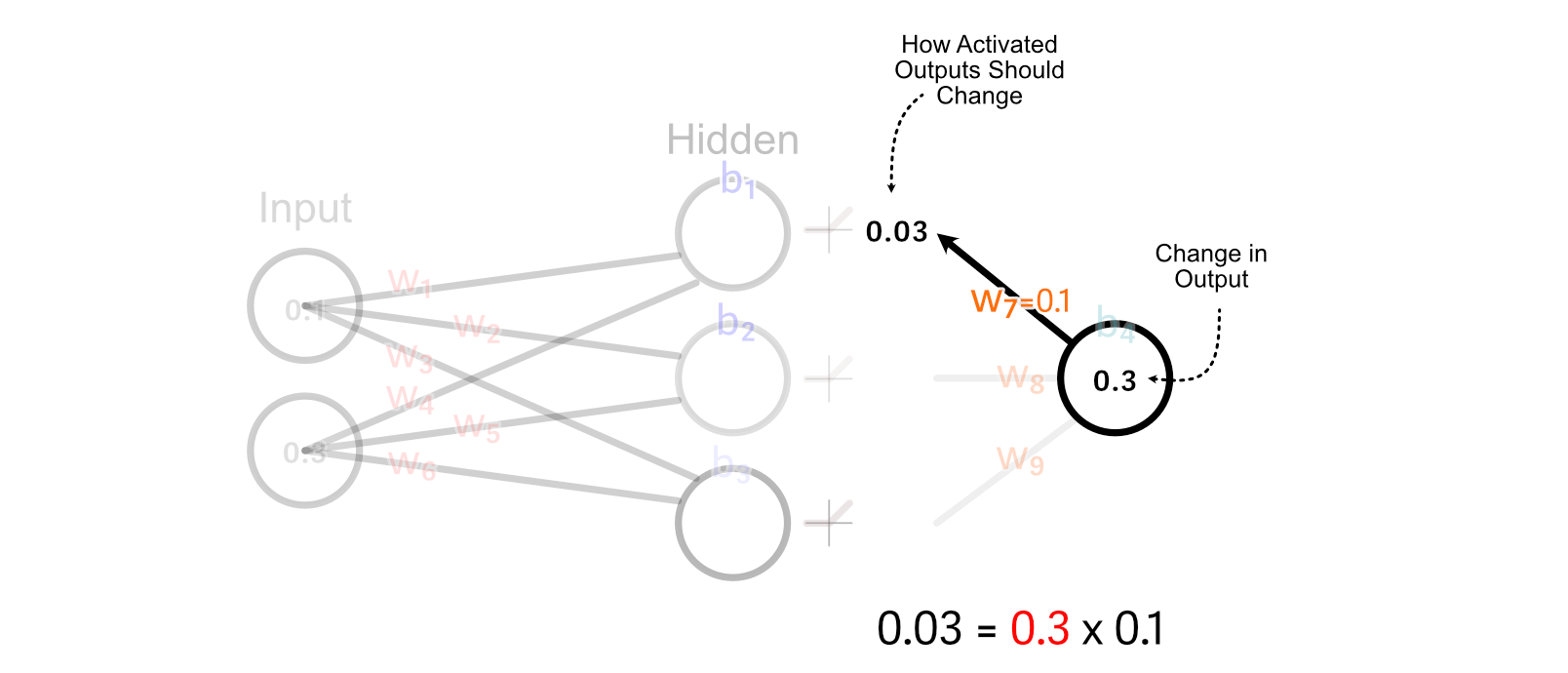
Now that we’ve calculated how the weights and bias of the output perceptron ought to change, we are able to “again propagate” our desired change in output via the mannequin. Let’s begin with again propagating so we are able to calculate how we should always replace w₁.
First, we calculate how the activated output of the of the primary hidden neuron ought to change. We do this by multiplying the change in output by w₇.
For values which might be larger than zero, ReLU merely multiplies these values by 1. So, for this instance, the change we would like the un-activated worth of the primary hidden neuron is the same as the specified change within the activated output
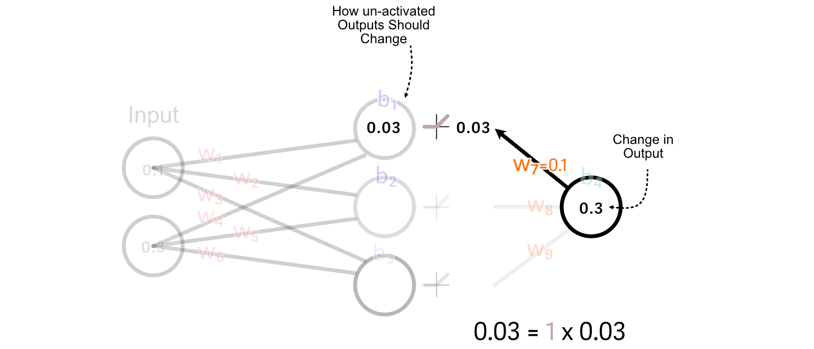
Recall that we calculated tips on how to replace w₇ primarily based on multiplying it’s enter by the change in its desired output. We are able to do the identical factor to calculate the change in w₁.
It’s essential to notice, we’re not truly updating any of the weights or biases all through this course of. Relatively, we’re taking a tally of how we should always replace every parameter, assuming no different parameters are up to date.
So, we are able to do these calculations to calculate all parameter adjustments.
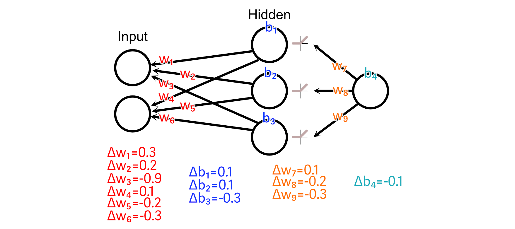
A basic concept of again propagation is named “Studying Price”, which considerations the dimensions of the adjustments we make to neural networks primarily based on a selected batch of information. To clarify why that is essential, I’d like to make use of an analogy.
Think about you went outdoors someday, and everybody carrying a hat gave you a humorous look. You most likely don’t need to soar to the conclusion that carrying hat = humorous look , however you could be a bit skeptical of individuals carrying hats. After three, 4, 5 days, a month, or perhaps a yr, if it looks as if the overwhelming majority of individuals carrying hats are supplying you with a humorous look, you might get thinking about {that a} sturdy development.
Equally, once we prepare a neural community, we don’t need to utterly change how the neural community thinks primarily based on a single coaching instance. Relatively, we would like every batch to solely incrementally change how the mannequin thinks. As we expose the mannequin to many examples, we might hope that the mannequin would study essential traits inside the knowledge.
After we’ve calculated how every parameter ought to change as if it have been the one parameter being up to date, we are able to multiply all these adjustments by a small quantity, like 0.001 , earlier than making use of these adjustments to the parameters. This small quantity is usually known as the “studying price”, and the precise worth it ought to have depends on the mannequin we’re coaching on. This successfully scales down our changes earlier than making use of them to the mannequin.
At this level we coated just about all the pieces one would wish to know to implement a neural community. Let’s give it a shot!

Implementing a Neural Community from Scratch
Usually, an information scientist would simply use a library like PyTorch to implement a neural community in just a few traces of code, however we’ll be defining a neural community from the bottom up utilizing NumPy, a numerical computing library.
First, let’s begin with a option to outline the construction of the neural community.
"""Blocking out the construction of the Neural Community
"""

import numpy as np

class SimpleNN:
    def __init__(self, structure):
        self.structure = structure
        self.weights = []
        self.biases = []

        # Initialize weights and biases
        np.random.seed(99)
        for i in vary(len(structure) - 1):
            self.weights.append(np.random.uniform(
                low=-1, excessive=1,
                measurement=(structure[i], structure[i+1])
            ))
            self.biases.append(np.zeros((1, structure[i+1])))

structure = [2, 64, 64, 64, 1]  # Two inputs, two hidden layers, one output
mannequin = SimpleNN(structure)

print('weight dimensions:')
for w in mannequin.weights:
    print(w.form)

print('nbias dimensions:')
for b in mannequin.biases:
    print(b.form)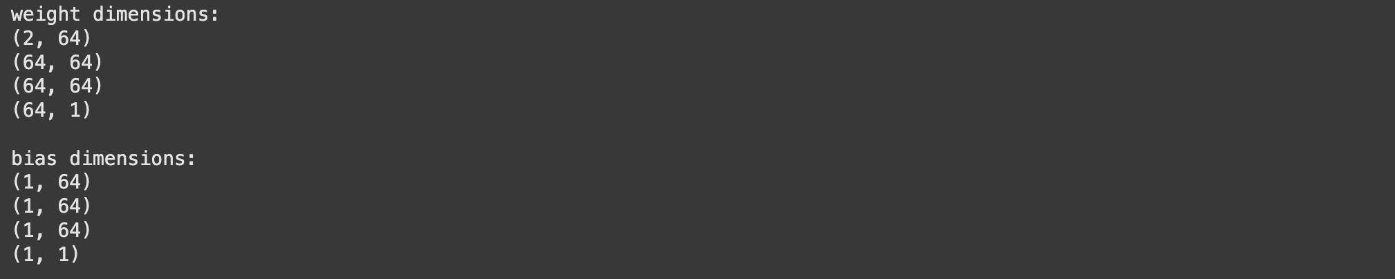
Whereas we sometimes draw neural networks as a dense net in actuality we signify the weights between their connections as matrices. That is handy as a result of matrix multiplication, then, is equal to passing knowledge via a neural community.
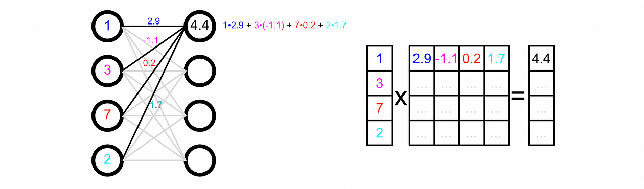
We are able to make our mannequin make a prediction primarily based on some enter by passing the enter via every layer.
"""Implementing the Ahead Cross
"""

import numpy as np

class SimpleNN:
    def __init__(self, structure):
        self.structure = structure
        self.weights = []
        self.biases = []

        # Initialize weights and biases
        np.random.seed(99)
        for i in vary(len(structure) - 1):
            self.weights.append(np.random.uniform(
                low=-1, excessive=1,
                measurement=(structure[i], structure[i+1])
            ))
            self.biases.append(np.zeros((1, structure[i+1])))

    @staticmethod
    def relu(x):
        #implementing the relu activation operate
        return np.most(0, x)

    def ahead(self, X):
        #iterating via all layers
        for W, b in zip(self.weights, self.biases):

            #making use of the load and bias of the layer
            X = np.dot(X, W) + b

            #doing ReLU for all however the final layer
            if W just isn't self.weights[-1]:
                X = self.relu(X)

        #returning the consequence
        return X

    def predict(self, X):
        y = self.ahead(X)
        return y.flatten()

#defining a mannequin
structure = [2, 64, 64, 64, 1]  # Two inputs, two hidden layers, one output
mannequin = SimpleNN(structure)

# Generate predictions
prediction = mannequin.predict(np.array([0.1,0.2]))
print(prediction)
We’d like to have the ability to prepare this mannequin, and to try this we’ll first want an issue to coach the mannequin on. I outlined a random operate that takes in two inputs and leads to an output:
"""Defining what we would like the mannequin to study
"""
import numpy as np
import matplotlib.pyplot as plt

# Outline a random operate with two inputs
def random_function(x, y):
    return (np.sin(x) + x * np.cos(y) + y + 3**(x/3))

# Generate a grid of x and y values
x = np.linspace(-10, 10, 100)
y = np.linspace(-10, 10, 100)
X, Y = np.meshgrid(x, y)

# Compute the output of the random operate
Z = random_function(X, Y)

# Create a 2D plot
plt.determine(figsize=(8, 6))
contour = plt.contourf(X, Y, Z, cmap='viridis')
plt.colorbar(contour, label='Operate Worth')
plt.title('2D Plot of Goal Operate')
plt.xlabel('X-axis')
plt.ylabel('Y-axis')
plt.present()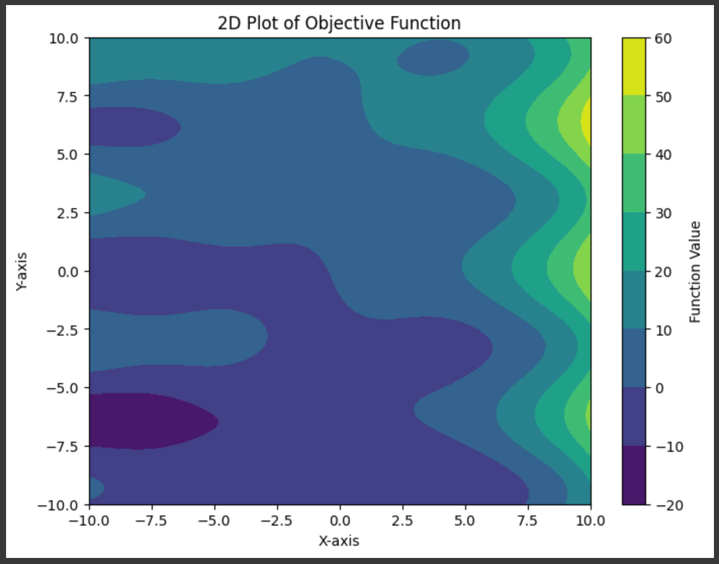
In the actual world we wouldn’t know the underlying operate. We are able to mimic that actuality by making a dataset consisting of random factors:
import numpy as np
import pandas as pd
import matplotlib.pyplot as plt

# Outline a random operate with two inputs
def random_function(x, y):
    return (np.sin(x) + x * np.cos(y) + y + 3**(x/3))

# Outline the variety of random samples to generate
n_samples = 1000

# Generate random X and Y values inside a specified vary
x_min, x_max = -10, 10
y_min, y_max = -10, 10

# Generate random values for X and Y
X_random = np.random.uniform(x_min, x_max, n_samples)
Y_random = np.random.uniform(y_min, y_max, n_samples)

# Consider the random operate on the generated X and Y values
Z_random = random_function(X_random, Y_random)

# Create a dataset
dataset = pd.DataFrame({
    'X': X_random,
    'Y': Y_random,
    'Z': Z_random
})

# Show the dataset
print(dataset.head())

# Create a 2D scatter plot of the sampled knowledge
plt.determine(figsize=(8, 6))
scatter = plt.scatter(dataset['X'], dataset['Y'], c=dataset['Z'], cmap='viridis', s=10)
plt.colorbar(scatter, label='Operate Worth')
plt.title('Scatter Plot of Randomly Sampled Information')
plt.xlabel('X-axis')
plt.ylabel('Y-axis')
plt.present()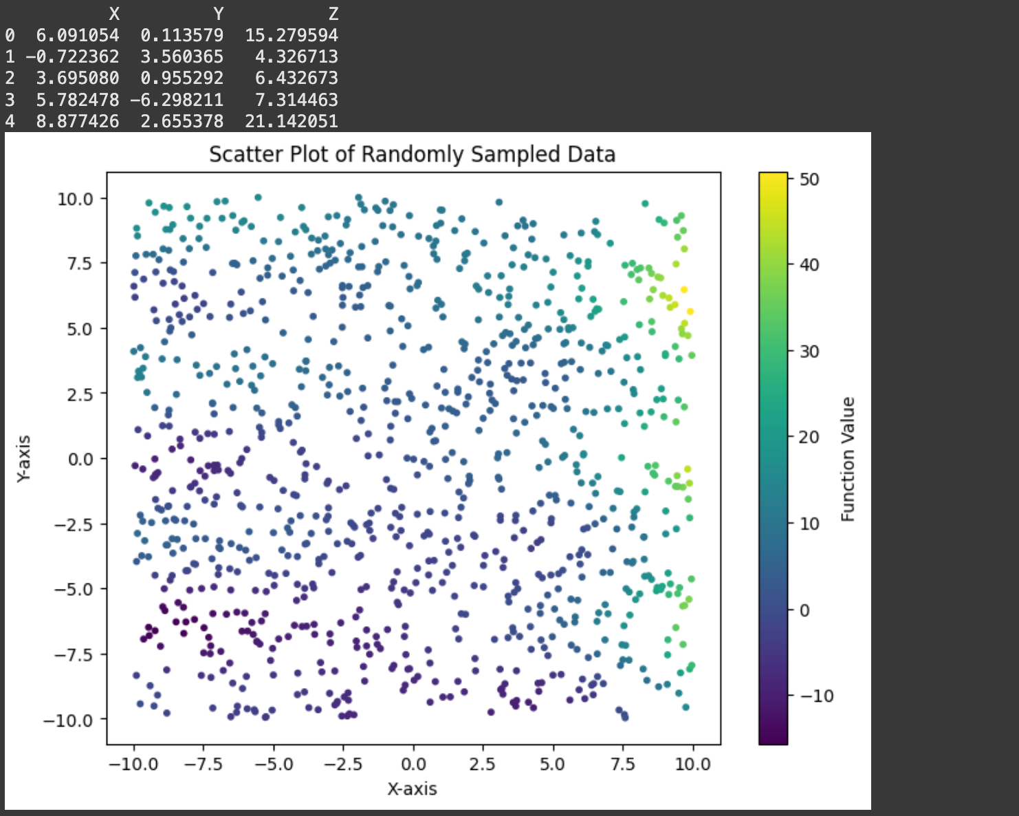
Recall that the again propagation algorithm updates parameters primarily based on what occurs in a ahead cross. So, earlier than we implement backpropagation itself, let’s maintain monitor of some essential values within the ahead cross: The inputs and outputs of every perceptron all through the mannequin.
import numpy as np

class SimpleNN:
    def __init__(self, structure):
        self.structure = structure
        self.weights = []
        self.biases = []

        #preserving monitor of those values on this code block
        #so we are able to observe them
        self.perceptron_inputs = None
        self.perceptron_outputs = None

        # Initialize weights and biases
        np.random.seed(99)
        for i in vary(len(structure) - 1):
            self.weights.append(np.random.uniform(
                low=-1, excessive=1,
                measurement=(structure[i], structure[i+1])
            ))
            self.biases.append(np.zeros((1, structure[i+1])))

    @staticmethod
    def relu(x):
        return np.most(0, x)

    def ahead(self, X):
        self.perceptron_inputs = [X]
        self.perceptron_outputs = []

        for W, b in zip(self.weights, self.biases):
            Z = np.dot(self.perceptron_inputs[-1], W) + b
            self.perceptron_outputs.append(Z)

            if W is self.weights[-1]:  # Final layer (output)
                A = Z  # Linear output for regression
            else:
                A = self.relu(Z)
            self.perceptron_inputs.append(A)

        return self.perceptron_inputs, self.perceptron_outputs

    def predict(self, X):
        perceptron_inputs, _ = self.ahead(X)
        return perceptron_inputs[-1].flatten()

#defining a mannequin
structure = [2, 64, 64, 64, 1]  # Two inputs, two hidden layers, one output
mannequin = SimpleNN(structure)

# Generate predictions
prediction = mannequin.predict(np.array([0.1,0.2]))

#trying via vital optimization values
for i, (inpt, outpt) in enumerate(zip(mannequin.perceptron_inputs, mannequin.perceptron_outputs[:-1])):
    print(f'layer {i}')
    print(f'enter: {inpt.form}')
    print(f'output: {outpt.form}')
    print('')

print('Closing Output:')
print(mannequin.perceptron_outputs[-1].form)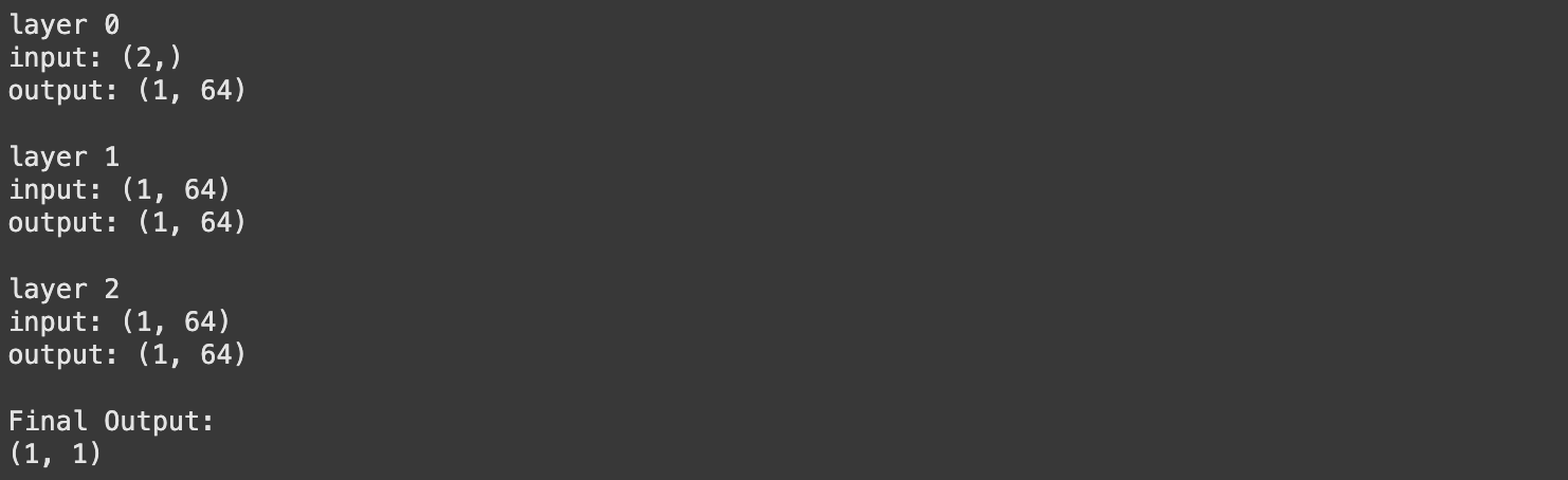
Now that we now have a report saved of vital middleman worth inside the community, we are able to use these values, together with the error of a mannequin for a selected prediction, to calculate the adjustments we should always make to the mannequin.
import numpy as np

class SimpleNN:
    def __init__(self, structure):
        self.structure = structure
        self.weights = []
        self.biases = []

        # Initialize weights and biases
        np.random.seed(99)
        for i in vary(len(structure) - 1):
            self.weights.append(np.random.uniform(
                low=-1, excessive=1,
                measurement=(structure[i], structure[i+1])
            ))
            self.biases.append(np.zeros((1, structure[i+1])))

    @staticmethod
    def relu(x):
        return np.most(0, x)

    @staticmethod
    def relu_as_weights(x):
        return (x > 0).astype(float)

    def ahead(self, X):
        perceptron_inputs = [X]
        perceptron_outputs = []

        for W, b in zip(self.weights, self.biases):
            Z = np.dot(perceptron_inputs[-1], W) + b
            perceptron_outputs.append(Z)

            if W is self.weights[-1]:  # Final layer (output)
                A = Z  # Linear output for regression
            else:
                A = self.relu(Z)
            perceptron_inputs.append(A)

        return perceptron_inputs, perceptron_outputs

    def backward(self, perceptron_inputs, perceptron_outputs, goal):
        weight_changes = []
        bias_changes = []

        m = len(goal)
        dA = perceptron_inputs[-1] - goal.reshape(-1, 1)  # Output layer gradient

        for i in reversed(vary(len(self.weights))):
            dZ = dA if i == len(self.weights) - 1 else dA * self.relu_as_weights(perceptron_outputs[i])
            dW = np.dot(perceptron_inputs[i].T, dZ) / m
            db = np.sum(dZ, axis=0, keepdims=True) / m
            weight_changes.append(dW)
            bias_changes.append(db)

            if i > 0:
                dA = np.dot(dZ, self.weights[i].T)

        return listing(reversed(weight_changes)), listing(reversed(bias_changes))

    def predict(self, X):
        perceptron_inputs, _ = self.ahead(X)
        return perceptron_inputs[-1].flatten()

#defining a mannequin
structure = [2, 64, 64, 64, 1]  # Two inputs, two hidden layers, one output
mannequin = SimpleNN(structure)

#defining a pattern enter and goal output
enter = np.array([[0.1,0.2]])
desired_output = np.array([0.5])

#doing ahead and backward cross to calculate adjustments
perceptron_inputs, perceptron_outputs = mannequin.ahead(enter)
weight_changes, bias_changes = mannequin.backward(perceptron_inputs, perceptron_outputs, desired_output)

#smaller numbers for printing
np.set_printoptions(precision=2)

for i, (layer_weights, layer_biases, layer_weight_changes, layer_bias_changes)
in enumerate(zip(mannequin.weights, mannequin.biases, weight_changes, bias_changes)):
    print(f'layer {i}')
    print(f'weight matrix: {layer_weights.form}')
    print(f'weight matrix adjustments: {layer_weight_changes.form}')
    print(f'bias matrix: {layer_biases.form}')
    print(f'bias matrix adjustments: {layer_bias_changes.form}')
    print('')

print('The load and weight change matrix of the second layer:')
print('weight matrix:')
print(mannequin.weights[1])
print('change matrix:')
print(weight_changes[1])
That is most likely probably the most complicated implementation step, so I need to take a second to dig via a few of the particulars. The elemental concept is strictly as we described in earlier sections. We’re iterating over all layers, from again to entrance, and calculating what change to every weight and bias would lead to a greater output.
# calculating output error
dA = perceptron_inputs[-1] - goal.reshape(-1, 1)

#a scaling issue for the batch measurement.
#you need adjustments to be a mean throughout all batches
#so we divide by m as soon as we have aggregated all adjustments.
m = len(goal)

for i in reversed(vary(len(self.weights))):
  dZ = dA #simplified for now

  # calculating change to weights
  dW = np.dot(perceptron_inputs[i].T, dZ) / m
  # calculating change to bias
  db = np.sum(dZ, axis=0, keepdims=True) / m

  # preserving monitor of required adjustments
  weight_changes.append(dW)
  bias_changes.append(db)
  ...
Calculating the change to bias is fairly straight ahead. In the event you take a look at how the output of a given neuron ought to have impacted all future neurons, you’ll be able to add up all these values (that are each optimistic and detrimental) to get an concept of if the neuron ought to be biased in a optimistic or detrimental course.
The way in which we calculate the change to weights, by utilizing matrix multiplication, is a little more mathematically complicated.
dW = np.dot(perceptron_inputs[i].T, dZ) / mPrincipally, this line says that the change within the weight ought to be equal to the worth going into the perceptron, occasions how a lot the output ought to have modified. If a perceptron had a giant enter, the change to its outgoing weights ought to be a big magnitude, if the perceptron had a small enter, the change to its outgoing weights shall be small. Additionally, if a weight factors in direction of an output which ought to change quite a bit, the load ought to change quite a bit.
There may be one other line we should always focus on in our again propagation implement.
dZ = dA if i == len(self.weights) - 1 else dA * self.relu_as_weights(perceptron_outputs[i])On this explicit community, there are activation features all through the community, following all however the last output. Once we do again propagation, we have to back-propagate via these activation features in order that we are able to replace the neurons which lie earlier than them. We do that for all however the final layer, which doesn’t have an activation operate, which is why dZ = dA if i == len(self.weights) - 1 .
In fancy math communicate we might name this a by-product, however as a result of I don’t need to get into calculus, I known as the operate relu_as_weights . Principally, we are able to deal with every of our ReLU activations as one thing like a tiny neural community, who’s weight is a operate of the enter. If the enter of the ReLU activation operate is lower than zero, then that’s like passing that enter via a neural community with a weight of zero. If the enter of ReLU is larger than zero, then that’s like passing the enter via a neural netowork with a weight of 1.
That is precisely what the relu_as_weights operate does.
def relu_as_weights(x):
        return (x > 0).astype(float)
Utilizing this logic we are able to deal with again propagating via ReLU similar to we again propagate via the remainder of the neural community.
Once more, I’ll be protecting this idea from a extra strong mathematical potential quickly, however that’s the important concept from a conceptual perspective.
Now that we now have the ahead and backward cross carried out, we are able to implement coaching the mannequin.
import numpy as np

class SimpleNN:
    def __init__(self, structure):
        self.structure = structure
        self.weights = []
        self.biases = []

        # Initialize weights and biases
        np.random.seed(99)
        for i in vary(len(structure) - 1):
            self.weights.append(np.random.uniform(
                low=-1, excessive=1,
                measurement=(structure[i], structure[i+1])
            ))
            self.biases.append(np.zeros((1, structure[i+1])))

    @staticmethod
    def relu(x):
        return np.most(0, x)

    @staticmethod
    def relu_as_weights(x):
        return (x > 0).astype(float)

    def ahead(self, X):
        perceptron_inputs = [X]
        perceptron_outputs = []

        for W, b in zip(self.weights, self.biases):
            Z = np.dot(perceptron_inputs[-1], W) + b
            perceptron_outputs.append(Z)

            if W is self.weights[-1]:  # Final layer (output)
                A = Z  # Linear output for regression
            else:
                A = self.relu(Z)
            perceptron_inputs.append(A)

        return perceptron_inputs, perceptron_outputs

    def backward(self, perceptron_inputs, perceptron_outputs, y_true):
        weight_changes = []
        bias_changes = []

        m = len(y_true)
        dA = perceptron_inputs[-1] - y_true.reshape(-1, 1)  # Output layer gradient

        for i in reversed(vary(len(self.weights))):
            dZ = dA if i == len(self.weights) - 1 else dA * self.relu_as_weights(perceptron_outputs[i])
            dW = np.dot(perceptron_inputs[i].T, dZ) / m
            db = np.sum(dZ, axis=0, keepdims=True) / m
            weight_changes.append(dW)
            bias_changes.append(db)

            if i > 0:
                dA = np.dot(dZ, self.weights[i].T)

        return listing(reversed(weight_changes)), listing(reversed(bias_changes))

    def update_weights(self, weight_changes, bias_changes, lr):
        for i in vary(len(self.weights)):
            self.weights[i] -= lr * weight_changes[i]
            self.biases[i] -= lr * bias_changes[i]

    def prepare(self, X, y, epochs, lr=0.01):
        for epoch in vary(epochs):
            perceptron_inputs, perceptron_outputs = self.ahead(X)
            weight_changes, bias_changes = self.backward(perceptron_inputs, perceptron_outputs, y)
            self.update_weights(weight_changes, bias_changes, lr)

            if epoch % 20 == 0 or epoch == epochs - 1:
                loss = np.imply((perceptron_inputs[-1].flatten() - y) ** 2)  # MSE
                print(f"EPOCH {epoch}: Loss = {loss:.4f}")

    def predict(self, X):
        perceptron_inputs, _ = self.ahead(X)
        return perceptron_inputs[-1].flatten()
The prepare operate:
- iterates via all the information some variety of occasions (outlined by
epoch) - passes the information via a ahead cross
- calculates how the weights and biases ought to change
- updates the weights and biases, by scaling their adjustments by the training price (
lr)
And thus we’ve carried out a neural community! Let’s prepare it.
Coaching and Evaluating the Neural Community.
Recall that we outlined an arbitrary 2D operate we wished to learn to emulate,
and we sampled that area with some variety of factors, which we’re utilizing to coach the mannequin.

Earlier than feeding this knowledge into our mannequin, it’s very important that we first “normalize” the information. Sure values of the dataset are very small or very massive, which might make coaching a neural community very troublesome. Values inside the neural community can rapidly develop to absurdly massive values, or diminish to zero, which might inhibit coaching. Normalization squashes all of our inputs, and our desired outputs, right into a extra cheap vary averaging round zero with a standardized distribution known as a “regular” distribution.
# Flatten the information
X_flat = X.flatten()
Y_flat = Y.flatten()
Z_flat = Z.flatten()

# Stack X and Y as enter options
inputs = np.column_stack((X_flat, Y_flat))
outputs = Z_flat

# Normalize the inputs and outputs
inputs_mean = np.imply(inputs, axis=0)
inputs_std = np.std(inputs, axis=0)
outputs_mean = np.imply(outputs)
outputs_std = np.std(outputs)

inputs = (inputs - inputs_mean) / inputs_std
outputs = (outputs - outputs_mean) / outputs_std
If we need to get again predictions within the precise vary of information from our authentic dataset, we are able to use these values to primarily “un-squash” the information.
As soon as we’ve executed that, we are able to outline and prepare our mannequin.
# Outline the structure: [input_dim, hidden1, ..., output_dim]
structure = [2, 64, 64, 64, 1]  # Two inputs, two hidden layers, one output
mannequin = SimpleNN(structure)

# Prepare the mannequin
mannequin.prepare(inputs, outputs, epochs=2000, lr=0.001)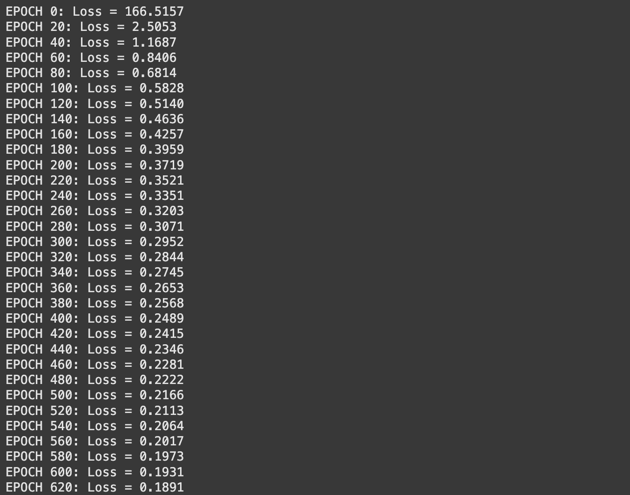
Then we are able to visualize the output of the neural community’s prediction vs the precise operate.
import matplotlib.pyplot as plt

# Reshape predictions to grid format for visualization
Z_pred = mannequin.predict(inputs) * outputs_std + outputs_mean
Z_pred = Z_pred.reshape(X.form)

# Plot comparability of the true operate and the mannequin predictions
fig, axes = plt.subplots(1, 2, figsize=(14, 6))

# Plot the true operate
axes[0].contourf(X, Y, Z, cmap='viridis')
axes[0].set_title("True Operate")
axes[0].set_xlabel("X-axis")
axes[0].set_ylabel("Y-axis")
axes[0].colorbar = plt.colorbar(axes[0].contourf(X, Y, Z, cmap='viridis'), ax=axes[0], label="Operate Worth")

# Plot the expected operate
axes[1].contourf(X, Y, Z_pred, cmap='plasma')
axes[1].set_title("NN Predicted Operate")
axes[1].set_xlabel("X-axis")
axes[1].set_ylabel("Y-axis")
axes[1].colorbar = plt.colorbar(axes[1].contourf(X, Y, Z_pred, cmap='plasma'), ax=axes[1], label="Operate Worth")

plt.tight_layout()
plt.present()
This did an okay job, however not as nice as we would like. That is the place loads of knowledge scientists spend their time, and there are a ton of approaches to creating a neural community match a sure downside higher. Some apparent ones are:
- use extra knowledge
- mess around with the training price
- prepare for extra epochs
- change the construction of the mannequin
It’s fairly simple for us to crank up the quantity of information we’re coaching on. Let’s see the place that leads us. Right here I’m sampling our dataset 10,000 occasions, which is 10x extra coaching samples than our earlier dataset.

After which I educated the mannequin similar to earlier than, besides this time it took quite a bit longer as a result of every epoch now analyses 10,000 samples somewhat than 1,000.
# Outline the structure: [input_dim, hidden1, ..., output_dim]
structure = [2, 64, 64, 64, 1]  # Two inputs, two hidden layers, one output
mannequin = SimpleNN(structure)

# Prepare the mannequin
mannequin.prepare(inputs, outputs, epochs=2000, lr=0.001)
I then rendered the output of this mannequin, the identical means I did earlier than, nevertheless it didn’t actually seem like the output received significantly better.

Wanting again on the loss output from coaching, it looks as if the loss remains to be steadily declining. Possibly I simply want to coach for longer. Let’s attempt that.
# Outline the structure: [input_dim, hidden1, ..., output_dim]
structure = [2, 64, 64, 64, 1]  # Two inputs, two hidden layers, one output
mannequin = SimpleNN(structure)

# Prepare the mannequin
mannequin.prepare(inputs, outputs, epochs=4000, lr=0.001)
The outcomes appear to be a bit higher, however they aren’t’ superb.

I’ll spare you the small print. I ran this just a few occasions, and I received some respectable outcomes, however by no means something 1 to 1. I’ll be protecting some extra superior approaches knowledge scientists use, like annealing and dropout, in future articles which can lead to a extra constant and higher output. Nonetheless, although, we made a neural community from scratch and educated it to do one thing, and it did a good job! Fairly neat!
Conclusion
On this article we averted calculus just like the plague whereas concurrently forging an understanding of Neural Networks. We explored their concept, a little bit bit concerning the math, the thought of again propagation, after which carried out a neural community from scratch. We then utilized a neural community to a toy downside, and explored a few of the easy concepts knowledge scientists make use of to truly prepare neural networks to be good at issues.
In future articles we’ll discover just a few extra superior approaches to Neural Networks, so keep tuned! For now, you could be excited by a extra thorough evaluation of Gradients, the elemental math behind again propagation.
You may additionally have an interest on this article, which covers coaching a neural community utilizing extra standard Information Science instruments like PyTorch.
AI for the Absolute Novice – Intuitively and Exhaustively Defined
Be a part of Intuitively and Exhaustively Defined
At IAEE you’ll find:
- Lengthy type content material, just like the article you simply learn
- Conceptual breakdowns of a few of the most cutting-edge AI subjects
- By-Hand walkthroughs of vital mathematical operations in AI
- Sensible tutorials and explainers


