Graph Coloring You Can See

Introduction

is the computational job of assigning colours to components of a graph in order that adjoining components by no means share the identical shade. It has functions in a number of domains, together with sports activities scheduling, cartography, avenue map navigation, and timetabling. It is usually of serious theoretical curiosity and a typical topic in university-level programs on graph concept, algorithms, and combinatorics.

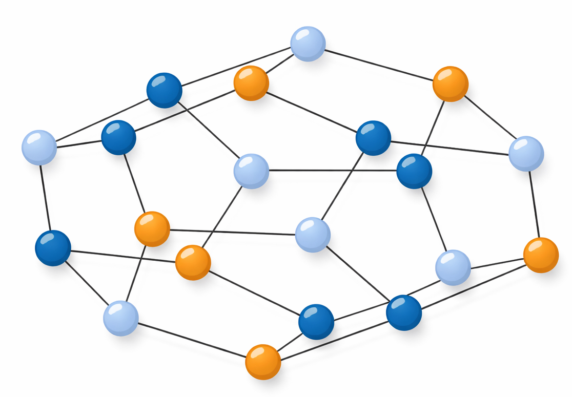
A graph is a mathematical construction comprising a set of nodes wherein some pairs of nodes are linked by edges. Given any graph,

• A node coloring is an task of colours to nodes so that every one pairs of nodes joined by edges have completely different colours,
• An edge coloring is an task of colours to edges so that every one edges that meet at a node have completely different colours,
• A face coloring of a graph is an task of colours to the faces of considered one of its planar embeddings (if such an embedding exists) in order that faces with frequent boundaries have completely different colours.

Examples of those ideas are proven within the photos above. Observe within the final instance that face colorings require nodes to be organized on the airplane in order that not one of the graph’s edges intersect. Consequently, they’re solely attainable for planar graphs. In distinction, node and edge colorings are attainable for all graphs. The purpose is to seek out colorings that use the minimal (optimum) variety of colours, which is an NP-hard drawback normally.

Articles on this discussion board (right here, right here and right here) have beforehand thought-about graph coloring, focusing totally on constructive heuristics for the node coloring drawback. On this article we contemplate node, edge, and face colorings and search to deliver the subject to life by means of detailed, visually partaking examples. To do that, we make use of the newly created GCol, library an open-source Python library constructed on prime of NetworkX. This library makes use of each exponential-time precise algorithms and polynomial-time heuristics.

The next Python code makes use of GCol to assemble and visualize node, edge, and face colorings of the graph seen above. A full itemizing of the code used to generate the photographs on this article is obtainable right here. An prolonged model of this text can also be out there right here.

import networkx as nx
import matplotlib.pyplot as plt
import gcol

G = nx.dodecahedral_graph()

# Generate and show a node coloring
c = gcol.node_coloring(G)
nx.draw_networkx(G, node_color=gcol.get_node_colors(G, c))
plt.present()

# Generate and show an edge coloring
c = gcol.edge_coloring(G)
nx.draw_networkx(G, edge_color=gcol.get_edge_colors(G, c))
plt.present()

# Generate node positions after which a face coloring
pos = nx.planar_layout(G)
c = gcol.face_coloring(G, pos)
gcol.draw_face_coloring(c, pos)
nx.draw_networkx(G, pos)
plt.present()

Node Coloring

Node coloring is essentially the most basic of the graph coloring issues. It’s because edge and face coloring issues can at all times be transformed into situations of the node coloring drawback. Particularly:

• An edge coloring of a graph may be achieved by coloring the nodes of its line graph,
• A face coloring of a planar graph may be discovered by coloring the nodes of its twin graph.

Edge and face coloring issues are subsequently particular circumstances of the node coloring drawback, regarding line graphs and planar graphs, respectively.

When visualizing node colorings, the spatial placement of the nodes impacts interpretability. Good node layouts can reveal structural patterns, clusters, and symmetries, whereas poor layouts can obscure them. One choice is to make use of force-directed strategies, which mannequin nodes as mutually repelling components and edges as springs. The tactic then adjusts the node positions to attenuate an power operate, balancing the attracting forces of edges and the repulsive forces from nodes. The purpose is to create an aesthetically pleasing format the place teams of associated nodes are shut, unrelated nodes are separated, and few edges intersect.

The colorings within the photos above reveal the consequences of various node positioning schemes. The primary instance makes use of randomly chosen positions, which appears to provide a moderately cluttered diagram. The second instance makes use of a force-directed methodology (particularly, NetworkX’s spring_layout() routine), leading to a extra logical format wherein communities and construction are extra obvious. GCol additionally permits nodes to be positioned primarily based on their colours. The third picture positions the nodes on the circumference of a circle, placing nodes of the identical shade in adjoining positions; the second arranges the nodes of every shade into columns. In these circumstances, the construction of the answer is extra obvious, and it’s simpler to watch that nodes of the identical shade can’t have edges between them.

Node colorings are normally simpler to show when the variety of edges and colours is small. Typically, the nodes even have a pure positioning that aids interpretation. Examples of such graphs are proven within the following photos. The primary three present examples of bipartite graphs (graphs that solely want two colours); the rest present graphs that require three colours.

Edge Coloring

Edge colorings require all edges ending at a selected node to have a distinct shade. In consequence, for any graph $G$ the minimal variety of colours wanted is at all times higher than or equal to $Delta(G)$, the place $Delta(G)$denotes the utmost diploma in $G$. For bipartite graphs, Konig’s theorem tells us that $Delta(G)$ colours are at all times enough.
Vizing’s theorem provides a extra basic consequence, stating that, for any graph $G$, not more than $Delta(G)+1$ colours are ever wanted.

Edge coloring has functions within the building of sports activities leagues, the place a set of groups are required to play one another over a collection of rounds. The primary instance above reveals a whole graph on six nodes, one node per staff. Right here, edges symbolize matches between groups, and every shade provides a single spherical within the schedule. Therefore, the “darkish blue” spherical includes matches between Groups 0 and 1, 2 and three, and 4 and 5, for instance. The opposite photos above present optimum edge colorings of two of the graphs seen earlier. These examples are harking back to crochet doily patterns or, maybe, Ojibwe dream catchers.

Edge colorings of two additional graphs are proven beneath. These assist for example how, utilizing edge coloring, walks round a graph may be specified by a beginning node and a sequence of colours that specify the order wherein edges are then adopted. This offers an alternate manner of specifying routes between places in avenue maps.

Face Coloring

The well-known four-color theorem states that face colorings of planar embeddings by no means require greater than 4 colours. This phenomenon was first famous in 1852 by Francis Guthrie whereas coloring a map of the counties of England; nevertheless, it could take over 100 years of analysis for it to be formally proved.

The above photos present face colorings of three graphs. Right here, nodes must be assumed wherever edges are seen to fulfill. On this determine, the central face of the Thomassen graph illustrates why 4 colours are typically wanted. As proven, this central face is adjoining to 5 surrounding faces. Collectively, these 5 faces kind an odd-length cycle, essentially requiring three completely different colours, so the central face should then be allotted to a fourth shade. A fifth shade won’t ever be wanted, although.

Face colorings usually want fewer than 4 colours, although. To reveal this, right here we contemplate a particular kind of graph generally known as Eulerian graph. That is merely a graph wherein the levels of all nodes are even. A planar graph is Eulerian if and provided that its twin graph is bipartite; consequently, the faces of Eulerian planar graphs can at all times be coloured utilizing two colours.

Examples of this are proven above the place, as required, all nodes have an excellent diploma. Sensible examples of this theorem may be seen in chess boards, Spirograph patterns, and plenty of types of Islamic and Celtic artwork, all of which characteristic underlying graphs which are each planar and Eulerian. Widespread tiling patterns involving sq., rectangular, or triangular tiles are additionally characterised by such graphs, as seen within the well-known “chequered” tiling type.

Two additional tiling patterns are proven beneath. The primary makes use of hexagonal tiles, the place the primary physique encompasses a repeating sample of three colours. The second instance reveals an optimum coloring of a not too long ago found aperiodic tiling sample. Right here, the 4 colors are distributed in a much less common method.

Our ultimate instance comes from an notorious spoof article from a 1975 situation of Scientific American. One of many false claims made on this article was {that a} graph had been found whose faces wanted at the very least 5 colours, subsequently disproving the 4 shade theorem. This graph is proven beneath, together with a 4 coloring.

Conclusions and Additional Assets

The article has reviewed and visualized a number of outcomes from the sector of graph coloring, making use of the open-source Python library GCol. At the beginning, we famous a number of essential sensible functions of this drawback, demonstrating that it’s helpful. This text has targeted on visible features, demonstrating that it’s also stunning.

The 4 shade theorem, originated from the remark that, when coloring territories on a geographical map, not more than 4 colours are wanted. Regardless of this, cartographers aren’t normally inquisitive about limiting themselves to only 4 colours. Certainly, it’s helpful for maps to additionally fulfill different constraints, similar to making certain that every one our bodies of water (and no land areas) are coloured blue, and that disjoint areas of the identical nation (similar to Alaska and the contiguous United States) obtain the identical shade. Such necessities may be modelled utilizing the precoloring and listing coloring issues, although they might effectively improve the required variety of colours past 4. Performance for these issues can also be included within the GCol library.

All supply code used to generate the figures may be discovered right here. An prolonged model of this text can be discovered right here. All figures have been generated by the creator.