Constructing A Trendy Dashboard with Python and Taipy

That is the third article in a brief sequence on creating knowledge dashboards utilizing the most recent Python-based growth instruments, Streamlit, Gradio and Taipy.

The supply knowledge set for every dashboard is identical, however saved in numerous codecs. As a lot as attainable, I’ll attempt to make the precise dashboard layouts for every device resemble one another and have the identical performance.

I’ve already written the Streamlit and Gradio variations. The Streamlit model will get its supply knowledge from a Postgres database. The Gradio and Taipy variations get their knowledge from a CSV file. Yow will discover hyperlinks to these different articles on the finish of this one.

What’s Taipy?

Taipy is a comparatively new Python-based net framework that turned distinguished a few years in the past. Based on its web site, Taipy is …

“… an open-source Python library for constructing production-ready front-end & back-end very quickly. No information of net growth is required!“

The audience for Taipy is knowledge scientists, machine studying practitioners and knowledge engineers who could not have in depth expertise creating front-end functions, however are sometimes fluent in Python. Taipy makes it fairly simple to create front-ends utilizing Python, in order that’s a win-win.

You may get began utilizing Taipy without cost. If you have to use it as a part of an enterprise, with devoted help and scalability, paid plans can be found on a month-to-month or yearly foundation. Their web site offers extra data, which I’ll hyperlink to on the finish of this text.

Why use Taipy over Gradio or Streamlit?

As I’ve proven on this and the opposite two articles, you possibly can develop very comparable output utilizing all three frameworks, so it begs the query of why use one over the opposite. 

Whereas Gradio excels at rapidly creating ML demos and Streamlit is sensible for interactive knowledge exploration, they each function on a precept of simplicity that may develop into a limitation as your software’s ambition grows. Taipy enters the image when your mission must graduate from a easy script or demo into a sturdy, performant, and maintainable software.

It’s best to strongly take into account selecting Taipy over Streamlit/Gradio if,

• Your app’s efficiency is crucial
• Your single script file is turning into unmanageably lengthy and sophisticated.
• You must construct multi-page functions with complicated navigation.
• Your software requires “what-if” situation evaluation or complicated pipeline execution.
• You might be constructing a manufacturing device for enterprise customers, not simply an inner exploratory dashboard.
• You might be working in a workforce and wish a clear, maintainable codebase.

Briefly, select Gradio for demos. Select Streamlit for interactive exploration. Select Taipy if you’re able to construct high-performance, scalable, and production-grade enterprise knowledge functions.

What we’ll develop

We’re creating a knowledge dashboard. Our supply knowledge shall be a single CSV file containing 100,000 artificial gross sales data.

The precise supply of the info isn’t that essential. It may simply as simply be saved as a Parquet file, in SQLite or Postgres, or any database you possibly can hook up with.

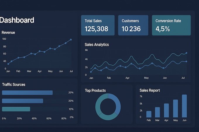
That is what our ultimate dashboard will seem like.

There are 4 essential sections.

• The highest row permits the consumer to pick particular begin and finish dates and/or product classes utilizing date pickers and a drop-down record, respectively.
• The second row, “Key Metrics,“ offers a top-level abstract of the chosen knowledge.
• The Visualisations part permits the consumer to pick one in every of three graphs to show the enter dataset.
• The Uncooked Knowledge part is strictly what it claims to be. This tabular illustration of the chosen knowledge successfully views the underlying CSV knowledge file.

Utilizing the dashboard is straightforward. Initially, stats for the entire knowledge set are displayed. The consumer can then slim the info focus utilizing the three alternative fields on the high of the show. The graphs, key metrics, and uncooked knowledge sections dynamically replace to replicate the consumer’s decisions.

The supply knowledge

As talked about, the dashboard’s supply knowledge is contained in a single comma-separated values (CSV) file. The information consists of 100,000 artificial sales-related data. Listed here are the primary ten data of the file.

+----------+------------+------------+----------------+------------+---------------+------------+----------+-------+--------------------+
| order_id | order_date | customer_id| customer_name  | product_id | product_names | classes | amount | worth | complete              |
+----------+------------+------------+----------------+------------+---------------+------------+----------+-------+--------------------+
| 0        | 01/08/2022 | 245        | Customer_884   | 201        | Smartphone    | Electronics| 3        | 90.02 | 270.06             |
| 1        | 19/02/2022 | 701        | Customer_1672  | 205        | Printer       | Electronics| 6        | 12.74 | 76.44              |
| 2        | 01/01/2017 | 184        | Customer_21720 | 208        | Pocket book      | Stationery | 8        | 48.35 | 386.8              |
| 3        | 09/03/2013 | 275        | Customer_23770 | 200        | Laptop computer        | Electronics| 3        | 74.85 | 224.55             |
| 4        | 23/04/2022 | 960        | Customer_23790 | 210        | Cupboard       | Workplace     | 6        | 53.77 | 322.62             |
| 5        | 10/07/2019 | 197        | Customer_25587 | 202        | Desk          | Workplace     | 3        | 47.17 | 141.51             |
| 6        | 12/11/2014 | 510        | Customer_6912  | 204        | Monitor       | Electronics| 5        | 22.5  | 112.5              |
| 7        | 12/07/2016 | 150        | Customer_17761 | 200        | Laptop computer        | Electronics| 9        | 49.33 | 443.97             |
| 8        | 12/11/2016 | 997        | Customer_23801 | 209        | Espresso Maker  | Electronics| 7        | 47.22 | 330.54             |
| 9        | 23/01/2017 | 151        | Customer_30325 | 207        | Pen           | Stationery | 6        | 3.5   | 21                 |
+----------+------------+------------+----------------+------------+---------------+------------+----------+-------+--------------------+

And right here is a few Python code you should utilize to generate a dataset. It utilises the NumPy and Pandas Python libraries, so be sure that each are put in earlier than working the code.

# generate the 100000 file CSV file
#
import polars as pl
import numpy as np
from datetime import datetime, timedelta

def generate(nrows: int, filename: str):
    names = np.asarray(
        [
            "Laptop",
            "Smartphone",
            "Desk",
            "Chair",
            "Monitor",
            "Printer",
            "Paper",
            "Pen",
            "Notebook",
            "Coffee Maker",
            "Cabinet",
            "Plastic Cups",
        ]
    )
    classes = np.asarray(
        [
            "Electronics",
            "Electronics",
            "Office",
            "Office",
            "Electronics",
            "Electronics",
            "Stationery",
            "Stationery",
            "Stationery",
            "Electronics",
            "Office",
            "Sundry",
        ]
    )
    product_id = np.random.randint(len(names), measurement=nrows)
    amount = np.random.randint(1, 11, measurement=nrows)
    worth = np.random.randint(199, 10000, measurement=nrows) / 100
    # Generate random dates between 2010-01-01 and 2023-12-31
    start_date = datetime(2010, 1, 1)
    end_date = datetime(2023, 12, 31)
    date_range = (end_date - start_date).days
    # Create random dates as np.array and convert to string format
    order_dates = np.array([(start_date + timedelta(days=np.random.randint(0, date_range))).strftime('%Y-%m-%d') for _ in range(nrows)])
    # Outline columns
    columns = {
        "order_id": np.arange(nrows),
        "order_date": order_dates,
        "customer_id": np.random.randint(100, 1000, measurement=nrows),
        "customer_name": [f"Customer_{i}" for i in np.random.randint(2**15, size=nrows)],
        "product_id": product_id + 200,
        "product_names": names[product_id],
        "classes": classes[product_id],
        "amount": amount,
        "worth": worth,
        "complete": worth * amount,
    }
    # Create Polars DataFrame and write to CSV with specific delimiter
    df = pl.DataFrame(columns)
    df.write_csv(filename, separator=',',include_header=True)  # Guarantee comma is used because the delimiter
# Generate 100,000 rows of knowledge with random order_date and save to CSV
generate(100_000, "/mnt/d/sales_data/sales_data.csv")

Putting in and utilizing Taipy

Putting in Taipy is straightforward, however earlier than coding, it’s finest follow to arrange a separate Python surroundings for all of your work. I exploit Miniconda for this objective, however be at liberty to make use of no matter technique fits your workflow. 

If you wish to observe the Miniconda route and don’t have already got it, you could first set up Miniconda.

As soon as the surroundings is created, swap to it utilizing the ‘activate’ command, after which run ‘pip set up’ to set up our required Python libraries.

#create our check surroundings
(base) C:Usersthoma>conda create -n taipy_dashboard python=3.12 -y

# Now activate it
(base) C:Usersthoma>conda activate taipy_dashboard

# Set up python libraries, and many others ...
(taipy_dashboard) C:Usersthoma>pip set up taipy pandas

The Code

I’ll break down the code into sections and clarify each as we proceed.

Part 1

from taipy.gui import Gui
import pandas as pd
import datetime

# Load CSV knowledge
csv_file_path = r"d:sales_datasales_data.csv"

attempt:
    raw_data = pd.read_csv(
        csv_file_path,
        parse_dates=["order_date"],
        dayfirst=True,
        low_memory=False  # Suppress dtype warning
    )
    if "income" not in raw_data.columns:
        raw_data["revenue"] = raw_data["quantity"] * raw_data["price"]
    print(f"Knowledge loaded efficiently: {raw_data.form[0]} rows")
besides Exception as e:
    print(f"Error loading CSV: {e}")
    raw_data = pd.DataFrame()

classes = ["All Categories"] + raw_data["categories"].dropna().distinctive().tolist()

# Outline the visualization choices as a correct record
chart_options = ["Revenue Over Time", "Revenue by Category", "Top Products"]

This script prepares gross sales knowledge to be used in our Taipy visualisation app. It does the next,

1. Imports the required exterior libraries and masses and preprocesses our supply knowledge from the enter CSV.
2. Calculates derived metrics like income.
3. Extracts related filtering choices (classes).
4. Defines obtainable visualisation choices.

Part 2

start_date = raw_data["order_date"].min().date() if not raw_data.empty else datetime.date(2020, 1, 1)
end_date = raw_data["order_date"].max().date() if not raw_data.empty else datetime.date(2023, 12, 31)
selected_category = "All Classes"
selected_tab = "Income Over Time"  # Set default chosen tab
total_revenue = "$0.00"
total_orders = 0
avg_order_value = "$0.00"
top_category = "N/A"
revenue_data = pd.DataFrame(columns=["order_date", "revenue"])
category_data = pd.DataFrame(columns=["categories", "revenue"])
top_products_data = pd.DataFrame(columns=["product_names", "revenue"])

def apply_changes(state):
    filtered_data = raw_data[
        (raw_data["order_date"] >= pd.to_datetime(state.start_date)) &
        (raw_data["order_date"] <= pd.to_datetime(state.end_date))
    ]
    if state.selected_category != "All Classes":
        filtered_data = filtered_data[filtered_data["categories"] == state.selected_category]

    state.revenue_data = filtered_data.groupby("order_date")["revenue"].sum().reset_index()
    state.revenue_data.columns = ["order_date", "revenue"]
    print("Income Knowledge:")
    print(state.revenue_data.head())

    state.category_data = filtered_data.groupby("classes")["revenue"].sum().reset_index()
    state.category_data.columns = ["categories", "revenue"]
    print("Class Knowledge:")
    print(state.category_data.head())

    state.top_products_data = (
        filtered_data.groupby("product_names")["revenue"]
        .sum()
        .sort_values(ascending=False)
        .head(10)
        .reset_index()
    )
    state.top_products_data.columns = ["product_names", "revenue"]
    print("Prime Merchandise Knowledge:")
    print(state.top_products_data.head())

    state.raw_data = filtered_data
    state.total_revenue = f"${filtered_data['revenue'].sum():,.2f}"
    state.total_orders = filtered_data["order_id"].nunique()
    state.avg_order_value = f"${filtered_data['revenue'].sum() / max(filtered_data['order_id'].nunique(), 1):,.2f}"
    state.top_category = (
        filtered_data.groupby("classes")["revenue"].sum().idxmax()
        if not filtered_data.empty else "N/A"
    )

def on_change(state, var_name, var_value):
    if var_name in {"start_date", "end_date", "selected_category", "selected_tab"}:
        print(f"State change detected: {var_name} = {var_value}")  # Debugging
        apply_changes(state)

def on_init(state):
    apply_changes(state)

import taipy.gui.builder as tgb

def get_partial_visibility(tab_name, selected_tab):
    return "block" if tab_name == selected_tab else "none"

Units the default begin and finish dates and preliminary class. Additionally, the preliminary chart shall be displayed as Income Over Time. Placeholder and preliminary values are additionally set for the next:-

• total_revenue. Set to "$0.00".
• total_orders. Set to 0.
• avg_order_value. Set to "$0.00".
• top_category. Set to "N/A".

Empty DataFrames are set for:-

• revenue_data. Columns are ["order_date", "revenue"].
• category_data. Columns are ["categories", "revenue"].
• top_products_data. Columns are ["product_names", "revenue"].

The apply_changes operate is outlined. This operate is triggered to replace the state when filters (reminiscent of date vary or class) are utilized. It updates the next:- 

• Time-series income traits.
• Income distribution throughout classes.
• The highest 10 merchandise by income.
• Abstract metrics (complete income, complete orders, common order worth, high class).

The on_change operate fires each time any of the user-selectable elements is modified

The on_init operate fires when the app is first run.

The get_partial_visibility operate determines the CSS show property for UI parts primarily based on the chosen tab.

Part 3

with tgb.Web page() as web page:
    tgb.textual content("# Gross sales Efficiency Dashboard", mode="md")
    
    # Filters part
    with tgb.half(class_name="card"):
        with tgb.format(columns="1 1 2"):  # Prepare parts in 3 columns
            with tgb.half():
                tgb.textual content("Filter From:")
                tgb.date("{start_date}")
            with tgb.half():
                tgb.textual content("To:")
                tgb.date("{end_date}")
            with tgb.half():
                tgb.textual content("Filter by Class:")
                tgb.selector(
                    worth="{selected_category}",
                    lov=classes,
                    dropdown=True,
                    width="300px"
                )
   
    # Metrics part
    tgb.textual content("## Key Metrics", mode="md")
    with tgb.format(columns="1 1 1 1"):
        with tgb.half(class_name="metric-card"):
            tgb.textual content("### Complete Income", mode="md")
            tgb.textual content("{total_revenue}")
        with tgb.half(class_name="metric-card"):
            tgb.textual content("### Complete Orders", mode="md")
            tgb.textual content("{total_orders}")
        with tgb.half(class_name="metric-card"):
            tgb.textual content("### Common Order Worth", mode="md")
            tgb.textual content("{avg_order_value}")
        with tgb.half(class_name="metric-card"):
            tgb.textual content("### Prime Class", mode="md")
            tgb.textual content("{top_category}")

    tgb.textual content("## Visualizations", mode="md")
    # Selector for visualizations with diminished width
    with tgb.half(type="width: 50%;"):  # Scale back width of the dropdown
        tgb.selector(
            worth="{selected_tab}",
            lov=["Revenue Over Time", "Revenue by Category", "Top Products"],
            dropdown=True,
            width="360px",  # Scale back width of the dropdown
        )

    # Conditional rendering of charts primarily based on selected_tab
    with tgb.half(render="{selected_tab == 'Income Over Time'}"):
        tgb.chart(
            knowledge="{revenue_data}",
            x="order_date",
            y="income",
            kind="line",
            title="Income Over Time",
        )

    with tgb.half(render="{selected_tab == 'Income by Class'}"):
        tgb.chart(
            knowledge="{category_data}",
            x="classes",
            y="income",
            kind="bar",
            title="Income by Class",
        )

    with tgb.half(render="{selected_tab == 'Prime Merchandise'}"):
        tgb.chart(
            knowledge="{top_products_data}",
            x="product_names",
            y="income",
            kind="bar",
            title="Prime Merchandise",
        )

    # Uncooked Knowledge Desk
    tgb.textual content("## Uncooked Knowledge", mode="md")
    tgb.desk(knowledge="{raw_data}")

This part of code defines the look and behavior of the general web page and is cut up up into a number of sub-sections

Web page Definition

tgp.web page(). Represents the dashboard’s essential container, defining the web page’s construction and parts.

Dashboard Structure

• Shows the title: “Gross sales Efficiency Dashboard” in Markdown mode (mode="md").

Filters Part

• Positioned inside a card-style half that makes use of a 3-column format – tgb.format(columns="1 1 2") — to rearrange the filters.

Filter Parts

1. Begin Date. A date picker tgb.date("{start_date}")for choosing the beginning of the date vary.
2. Finish Date. A date picker tgb.date("{end_date}") for selecting the top of the date vary.
3. Class Filter.

• A dropdown selector tgb.selector to filter knowledge by classes.
• Populated utilizing classes e.g., "All Classes" and obtainable classes from the dataset.

Key Metrics Part

Shows abstract statistics in 4 metric playing cards organized in a 4-column format:

• Complete Income. Reveals the total_revenue worth.
• Complete Orders. Shows the variety of distinctive orders (total_orders).
• Common Order Worth. Reveals the avg_order_value.
• Prime Class. Shows the title of the class contributing probably the most income.

Visualizations Part

• A drop-down selector permits customers to change between completely different visualisations (e.g., “Income Over Time,” “Income by Class,” “Prime Merchandise”).
• The dropdown width is diminished for a compact UI.

Conditional Rendering of Charts

• Income over time. Shows the road chart revenue_data displaying income traits over time.
• Income by class. Reveals the bar chart category_data to visualise income distribution throughout classes.
• Prime merchandise. Shows the bar chart top_products_data displaying the highest 10 merchandise by income.

Uncooked Knowledge Desk

• Shows the uncooked dataset in a tabular format.
• Dynamically updates primarily based on user-applied filters (e.g., date vary, class).

Part 4

Gui(web page).run(
    title="Gross sales Dashboard",
    dark_mode=False,
    debug=True,
    port="auto",
    allow_unsafe_werkzeug=True,
    async_mode="threading"
)

This ultimate, quick part renders the web page for show on a browser.

Operating the code

Gather all of the above code snippets and save them to a file, e.g taipy-app.py. Be sure your supply knowledge file is within the right location and referenced accurately in your code. You then run the module identical to some other Python code by typing this right into a command-line terminal.

python taipy-app.py

After a second or two, it’s best to see a browser window open along with your knowledge app displayed.

Abstract

On this article, I’ve tried to supply a complete information to constructing an interactive gross sales efficiency dashboard with Taipy utilizing a CSV file as its supply knowledge.

I defined that Taipy is a contemporary, Python-based open-source framework that simplifies the creation of data-driven dashboards and functions. I additionally offered some options on why you may need to use TaiPy over the opposite two widespread frameworks, Gradio and Streamlit.

The dashboard I developed permits customers to filter knowledge by date ranges and product classes, view key metrics reminiscent of complete income and top-performing classes, discover visualisations like income traits and high merchandise, and navigate via uncooked knowledge with pagination.

This information offers a complete implementation, overlaying your entire course of from creating pattern knowledge to creating Python features for querying knowledge, producing plots, and dealing with consumer enter. This step-by-step method demonstrates leverage Taipy’s capabilities to create user-friendly and dynamic dashboards, making it splendid for knowledge engineers and scientists who need to construct interactive knowledge functions.

Though I used a CSV file for my knowledge supply, modifying the code to make use of one other knowledge supply, reminiscent of a relational database administration system (RDBMS) like SQLite, must be easy.

For extra data on Taipy, their web site is https://taipy.io/

To view my different two TDS articles on constructing knowledge dashboards utilizing Gradio and Streamlit, click on the hyperlinks under.

Gradio dashboard

Streamlit dashboard