


Coaching a language mannequin is memory-intensive, not solely as a result of the mannequin itself is massive but additionally as a result of the lengthy sequences within the coaching knowledge batches. Coaching a mannequin with restricted reminiscence is difficult. On this article, you’ll study methods that allow mannequin coaching in memory-constrained environments. Particularly, you’ll find out about:
- Low-precision floating-point numbers and mixed-precision coaching
- Utilizing gradient checkpointing
Let’s get began!

Coaching a Mannequin with Restricted Reminiscence utilizing Combined Precision and Gradient Checkpointing
Picture by Meduana. Some rights reserved.
Overview
This text is split into three elements; they’re:
- Floating-point Numbers
- Computerized Combined Precision Coaching
- Gradient Checkpointing
Let’s get began!
Floating-Level Numbers
The default knowledge kind in PyTorch is the IEEE 754 32-bit floating-point format, also referred to as single precision. It’s not the one floating-point kind you should use. For instance, most CPUs help 64-bit double-precision floating-point, and GPUs usually help half-precision floating-point as nicely. The desk under lists some floating-point sorts:
| Knowledge Sort | PyTorch Sort | Whole Bits | Signal Bit | Exponent Bits | Mantissa Bits | Min Worth | Max Worth | eps |
|---|---|---|---|---|---|---|---|---|
| IEEE 754 double precision | torch.float64 |
64 | 1 | 11 | 52 | -1.79769e+308 | 1.79769e+308 | 2.22045e-16 |
| IEEE 754 single precision | torch.float32 |
32 | 1 | 8 | 23 | -3.40282e+38 | 3.40282e+38 | 1.19209e-07 |
| IEEE 754 half precision | torch.float16 |
16 | 1 | 5 | 10 | -65504 | 65504 | 0.000976562 |
| bf16 | torch.bfloat16 |
16 | 1 | 8 | 7 | -3.38953e+38 | 3.38953e+38 | 0.0078125 |
| fp8 (e4m3) | torch.float8_e4m3fn |
8 | 1 | 4 | 3 | -448 | 448 | 0.125 |
| fp8 (e5m2) | torch.float8_e5m2 |
8 | 1 | 5 | 2 | -57344 | 57344 | 0.25 |
| fp8 (e8m0) | torch.float8_e8m0fnu |
8 | 1 | 8 | 0 | 1.70141e+38 | 5.87747e-39 | 1.0 |
| fp6 (e3m2) | 6 | 1 | 3 | 2 | -28 | 28 | 0.25 | |
| fp6 (e2m3) | 6 | 1 | 2 | 3 | -7.5 | 7.5 | 0.125 | |
| fp4 (e2m1) | 4 | 1 | 2 | 1 | -6 | 6 |
Floating-point numbers are binary representations of actual numbers. Every consists of an indication bit, a number of bits for the exponent, and a number of other bits for the mantissa. They’re laid out as proven within the determine under. When sorted by their binary illustration, floating-point numbers retain their order by real-number worth.
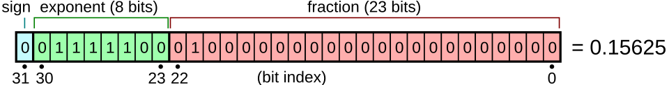
Floating-point quantity illustration. Determine from Wikimedia.
Totally different floating-point sorts have completely different ranges and precisions. Not every kind are supported by all {hardware}. For instance, fp4 is barely supported in Nvidia’s Blackwell structure. PyTorch helps just a few knowledge sorts. You may run the next code to print details about varied floating-point sorts:
|
1 2 3 4 5 6 7 8 9 10 11 12 13 14 15 16 17 18 19 20 21 22 23 24 25 26 |
import torch from tabulate import tabulate
# float sorts: float_types = [ torch.float64, torch.float32, torch.float16, torch.bfloat16, torch.float8_e4m3fn, torch.float8_e5m2, torch.float8_e8m0fnu, ]
# acquire finfo for every kind desk = [] for dtype in float_types: information = torch.finfo(dtype) attempt: typename = information.dtype besides: typename = str(dtype) desk.append([typename, info.max, info.min, info.smallest_normal, info.eps])
headers = [‘data type’, ‘max’, ‘min’, ‘smallest normal’, ‘eps’] print(tabulate(desk, headers=headers)) |
Take note of the min and max values for every kind, in addition to the eps worth. The min and max values point out the vary a kind can help (the dynamic vary). If you happen to practice a mannequin with such a kind, however the mannequin weights exceed this vary, you’ll get overflow or underflow, often inflicting the mannequin to output NaN or Inf. The eps worth is the smallest optimistic quantity such that the sort can differentiate between 1+eps and 1. It is a metric for precision. In case your mannequin’s gradient updates are smaller than eps, you’ll seemingly observe the vanishing gradient drawback.
Due to this fact, float32 is an efficient default alternative for deep studying: it has a large dynamic vary and excessive precision. Nonetheless, every float32 quantity requires 4 bytes of reminiscence. As a compromise, you should use float16 to avoid wasting reminiscence, however you’re prone to encounter overflow or underflow points because the dynamic vary is way smaller.
The Google Mind staff recognized this drawback and proposed bfloat16, a 16-bit floating-point format with the identical dynamic vary as float32. As a trade-off, the precision is an order of magnitude worse than float16. It seems that dynamic vary is extra essential than precision for deep studying, making bfloat16 extremely helpful.
If you create a tensor in PyTorch, you’ll be able to specify the information kind. For instance:
|
x = torch.tensor([1.0, 2.0, 3.0], dtype=torch.float16) print(x) |
There’s a simple approach to change the default to a unique kind, corresponding to bfloat16. That is useful for mannequin coaching. All you have to do is about the next line earlier than you create any mannequin or optimizer:
|
# set default dtype to bfloat16 torch.set_default_dtype(torch.bfloat16) |
Simply by doing this, you power all of your mannequin weights and gradients to be bfloat16 kind. This protects half of the reminiscence. Within the earlier article, you had been suggested to set the batch dimension to eight to suit a GPU with solely 12GB of VRAM. With bfloat16, you must be capable of set the batch dimension to 16.
Word that making an attempt to make use of 8-bit float or lower-precision sorts could not work. It is because you want {hardware} help and PyTorch to carry out the corresponding mathematical operations. You may attempt the next code (requires a CUDA gadget) and discover that you’ll want additional effort to function on 8-bit float:
|
1 2 3 4 5 6 7 8 9 10 11 12 13 14 15 16 17 18 |
dtype = torch.float8_e4m3fn
# Outline a tensor with float8 will see # NotImplementedError: “normal_kernel_cuda” not carried out for ‘Float8_e4m3fn’ x = torch.randn(16, 16, dtype=dtype, gadget=“cuda”)
# Create in float32 and convert to float8 works x = torch.randn(16, 16, gadget=“cuda”).to(dtype)
# However matmul shouldn’t be supported. You will note # NotImplementedError: “addmm_cuda” not carried out for ‘Float8_e4m3fn’ y = x @ x.T
# The right approach to run matrix multiplication on 8-bit float y = torch._scaled_mm(x, x.T, out_dtype=dtype, scale_a=torch.tensor(1.0, gadget=“cuda”), scale_b=torch.tensor(1.0, gadget=“cuda”)) print(y) |
Computerized Combined Precision Coaching
Coaching a mannequin with float16 could encounter points as a result of not all operations ought to be carried out at decrease precision. For instance, matrix multiplication is powerful in decrease precision, however discount operations, pooling, and a few activation capabilities require float32.
You may set the information kind manually for every part of your mannequin, however that is tedious since you should convert knowledge sorts between elements. A greater resolution is to make use of automated combined precision coaching in PyTorch.
PyTorch has a sub-library torch.amp that may routinely forged the information kind based mostly on the operation. Not all operations are carried out in the identical floating-point kind. If the operation is thought to be sturdy at decrease precision, this library will forged the tensors to that precision earlier than working the operation. Therefore the title “combined precision”. Utilizing decrease precision could not solely save reminiscence but additionally velocity up coaching. Some GPUs can run float16 operations at twice the velocity of float32.
If you practice a mannequin with torch.amp, all you have to do is run your ahead move beneath the context of torch.amp.autocast(). Sometimes, additionally, you will use a GradScaler to deal with gradient scaling. That is needed as a result of beneath low precision, you might encounter vanishing gradients because of the restricted precision of your floating-point kind. The GradScaler scales the gradient earlier than the backward move to forestall lack of gradient stream. In the course of the backward move, you must scale the gradient again for correct updates. This course of will be cumbersome as a result of you have to decide the right scale issue, which the GradScaler handles for you.
In comparison with the coaching loop from the earlier article, under is the way you sometimes use torch.amp to coach a mannequin:
|
1 2 3 4 5 6 7 8 9 10 11 12 13 14 15 16 17 18 19 20 21 22 23 24 25 26 27 28 29 30 31 32 33 |
...
# Examine if combined precision coaching is supported assert torch.amp.autocast_mode.is_autocast_available(“cuda”)
# Creates a GradScaler earlier than the coaching loop scaler = torch.amp.GradScaler(“cuda”, enabled=True)
# begin coaching for epoch in vary(begin_epoch, epochs): pbar = tqdm.tqdm(dataloader, desc=f“Epoch {epoch+1}/{epochs}”) for batch_id, batch in enumerate(pbar): # get batched knowledge input_ids, target_ids = batch # create consideration masks: causal masks + padding masks attn_mask = create_causal_mask(input_ids.form[1], gadget) + create_padding_mask(input_ids, PAD_TOKEN_ID, gadget) # with autocasting to bfloat16, run the ahead move with torch.autocast(device_type=“cuda”, dtype=torch.bfloat16): logits = mannequin(input_ids, attn_mask) loss = loss_fn(logits.view(–1, logits.dimension(–1)), target_ids.view(–1)) # backward with loss, scaled by the GradScaler optimizer.zero_grad() scaler.scale(loss).backward() # step the optimizer and test if the size has been up to date scaler.step(optimizer) old_scale = scaler.get_scale() scaler.replace() if scaler.get_scale() < old_scale: scheduler.step() pbar.set_postfix(loss=loss.merchandise()) pbar.replace(1) pbar.shut() |
Utilizing AMP autocasting is simple: hold the mannequin’s default precision at float32, then wrap the ahead move and loss computation with torch.autocast(). Underneath this context, all supported operations will run within the specified knowledge kind.
Upon getting the loss, let the GradScaler deal with the backward move. It should scale up the loss and replace the mannequin’s gradients. Nonetheless, this may increasingly trigger points if the scaling is simply too massive, leading to NaN or Inf gradients. Due to this fact, use scaler.step(optimizer) to step the optimizer, which verifies the gradients earlier than executing the optimizer step. If GradScaler decides to not step the optimizer, it’s going to cut back the size issue when replace() is named. Examine whether or not the size has been up to date to find out when you ought to step the scheduler.
Because the backward move makes use of scaled loss, when you use gradient clipping, you must unscale the gradients earlier than clipping. Right here’s tips on how to do it:
|
... # backward with loss, scaled by the GradScaler optimizer.zero_grad() scaler.scale(loss).backward() # unscaled the gradients and apply gradient clipping scaler.unscale_(optimizer) torch.nn.utils.clip_grad_norm_(mannequin.parameters(), 1.0) # step the optimizer and test if the size has been up to date scaler.step(optimizer) old_scale = scaler.get_scale() scaler.replace() if scaler.get_scale() < old_scale: scheduler.step() |
Usually, you don’t have to name scaler.unscale_() manually because it’s a part of the scaler.step(optimizer) name. Nonetheless, it’s essential to accomplish that when making use of gradient clipping in order that the clipping operate can observe the precise gradients.
Autocasting is automated, however the GradScaler maintains a state to trace the size issue. Due to this fact, whenever you checkpoint your mannequin, you must also save the scaler.state_dict(), simply as you’d save the optimizer state:
|
... # Loading checkpoint checkpoint = torch.load(“training_checkpoint.pth”) mannequin.load_state_dict(checkpoint[“model”]) optimizer.load_state_dict(checkpoint[“optimizer”]) scheduler.load_state_dict(checkpoint[“scheduler”]) scaler.load_state_dict(checkpoint[“scaler”])
# Saving checkpoint torch.save({ “mannequin”: mannequin.state_dict(), “optimizer”: optimizer.state_dict(), “scheduler”: scheduler.state_dict(), “scaler”: scaler.state_dict(), }, f“training_checkpoint.pth”) |
Gradient Checkpointing
If you practice a mannequin with half precision, you utilize half the reminiscence in comparison with 32-bit float. With mixed-precision coaching, you might use barely extra reminiscence as a result of not all operations run at decrease precision.
If you happen to nonetheless encounter reminiscence points, one other method trades time for reminiscence: gradient checkpointing. Recall that in deep studying, for a operate $y=f(mathbb{u})$ and $mathbb{u}=g(mathbb{x}))$, then
$$
frac{partial y}{partial mathbb{x}} = large(frac{partial mathbb{u}}{partial mathbb{x}}large)^prime frac{partial y}{partial mathbb{u}}
$$
the place $y$ is a scalar (often the loss metric), and $mathbb{u}$ and $mathbb{x}$ are vectors. The time period $frac{partial mathbb{u}}{partial mathbb{x}}$ is the Jacobian matrix of $mathbb{u}$ with respect to $mathbb{x}$.
The gradient $frac{partial y}{partial mathbb{x}}$ is required to replace $mathbb{x}$ however is dependent upon $frac{partial y}{partial mathbb{u}}$. Usually, whenever you run the ahead move, all intermediate outcomes corresponding to $mathbb{u}$ are saved in reminiscence in order that whenever you run the backward move, you’ll be able to readily compute the gradient $frac{partial y}{partial mathbb{u}}$. Nonetheless, this requires substantial reminiscence for deep networks.
Gradient checkpointing discards some intermediate outcomes. So long as $mathbb{u}=g(mathbb{x})$, you’ll be able to recompute $mathbb{u}$ from $mathbb{x}$ in the course of the backward move. This fashion, you don’t have to retailer $mathbb{u}$ in reminiscence, however it’s essential to compute $mathbb{u}$ twice: as soon as for the ahead move and as soon as for the backward move.
You may determine which intermediate outcomes to discard. Making use of gradient checkpointing to each two operations nonetheless requires storing many intermediate outcomes. Making use of it to bigger blocks saves extra reminiscence.
Referring to the mannequin from the earlier article, you’ll be able to wrap each transformer block with gradient checkpointing:
|
1 2 3 4 5 6 7 8 9 10 11 12 13 14 15 16 17 18 19 20 21 22 23 24 |
... class LlamaModel(nn.Module): def __init__(self, config: LlamaConfig) -> None: tremendous().__init__() self.rotary_emb = RotaryPositionEncoding( config.hidden_size // config.num_attention_heads, config.max_position_embeddings, )
self.embed_tokens = nn.Embedding(config.vocab_size, config.hidden_size) self.layers = nn.ModuleList([LlamaDecoderLayer(config) for _ in range(config.num_hidden_layers)]) self.norm = nn.RMSNorm(config.hidden_size, eps=1e–5)
def ahead(self, input_ids: Tensor, attn_mask: Tensor) -> Tensor: # Convert enter token IDs to embeddings hidden_states = self.embed_tokens(input_ids) # Course of by way of all transformer layers, then the ultimate norm layer for layer in self.layers: # Beforehand: # hidden_states = layer(hidden_states, rope=self.rotary_emb, attn_mask=attn_mask) hidden_states = torch.utils.checkpoint.checkpoint(layer, hidden_states, self.rotary_emb, attn_mask) hidden_states = self.norm(hidden_states) # Return the ultimate hidden states return hidden_states |
Just one line of code wants to vary: within the for-loop beneath the ahead() operate, as a substitute of calling the transformer block instantly, use torch.utils.checkpoint.checkpoint(). This runs the ahead move with gradient checkpointing, discarding all intermediate outcomes and retaining solely the block’s enter and output. In the course of the backward move, the intermediate outcomes are briefly recomputed utilizing the enter.
Additional readings
Beneath are some assets that you could be discover helpful:
Abstract
On this article, you discovered methods for coaching a language mannequin with restricted reminiscence. Particularly, you discovered that:
- A number of kinds of floating-point numbers exist, with some utilizing much less reminiscence than others.
- Combined-precision coaching routinely makes use of lower-precision floating-point numbers with out sacrificing accuracy on vital operations.
- Gradient checkpointing trades time for reminiscence throughout coaching.


