


On this article, you’ll discover ways to construct a textual content clustering pipeline by combining giant language mannequin embeddings with HDBSCAN, a density-based clustering algorithm, to mechanically uncover subjects in unlabeled textual content knowledge.
Matters we’ll cowl embody:
- Learn how to generate textual content embeddings for uncooked paperwork utilizing a pre-trained sentence-transformers mannequin.
- Learn how to cut back the dimensionality of these embeddings with UMAP to arrange them for clustering.
- Learn how to apply HDBSCAN to mechanically uncover matter clusters and visualize the outcomes.

Clustering Unstructured Textual content with LLM Embeddings and HDBSCAN
Introduction
The present period of Generative AI appears to primarily concentrate on chat interfaces and prompts, however the vary of functions of giant language fashions, or LLMs for brief, shouldn’t be restricted to only that. Certainly, one among their strongest downstream talents consists of turning uncooked, messy, unstructured textual content into semantically wealthy mathematical representations known as embeddings. As soon as that’s achieved, we are able to use these textual content representations for quite a lot of machine studying use circumstances, with clustering being no exception.
Particularly, embeddings could be mixed with superior, density-based clustering methods like HDBSCAN, permitting because of this for the invention of hidden subjects, patterns, or classes in your assortment of textual content paperwork: all with out the necessity for prior labeling.
This text reveals tips on how to assemble a text-based clustering pipeline from scratch. We are going to use a freely accessible dataset containing textual content situations, in addition to an open-source LLM that has been skilled for producing embeddings — i.e. a so-called embedding mannequin. The icing on the cake: we’ll use free and useful, fashionable Python libraries offering implementations of clustering algorithms like HDBSCAN.
Step-by-Step Walkthrough
First, let’s begin by putting in the important thing Python libraries we’ll want:
- Sentence transformers, to load a pre-trained LLM for embedding technology from Hugging Face — you’ll want a Hugging Face API key, additionally known as an entry token, to have the ability to load the mannequin.
- Umap-learn, to use an algorithm to scale back the dimensionality of embeddings.
Likewise, if you’re engaged on an area IDE as a substitute of a cloud pocket book setting and don’t have scikit-learn and pandas, you might want to put in them too.
|
!pip set up sentence–transformers umap–be taught |
Now we begin the coding half by getting some contemporary knowledge. The fetch_20newsgroups operate, which fetches a dataset containing texts from categorized information articles, will do. Notice that despite the fact that the dataset accommodates labels, we’ll omit them, as we’re pretending to not know this data for the sake of clustering these knowledge situations into teams primarily based on similarity. Additionally, we pattern down the dataset to 150 situations, which can be consultant sufficient for our instance.
|
import pandas as pd from sklearn.datasets import fetch_20newsgroups
# Fetching a extremely focused subset of information (~150-200 docs) classes = [‘sci.space’, ‘sci.med’, ‘rec.autos’] newsgroups = fetch_20newsgroups(subset=‘practice’, classes=classes, take away=(‘headers’, ‘footers’, ‘quotes’))
# Sampling down right into a consultant, illustrative subset df = pd.DataFrame({‘textual content’: newsgroups.knowledge, ‘true_label’: newsgroups.goal}) df = df[df[‘text’].str.strip().str.len() > 100].pattern(150, random_state=42).reset_index(drop=True)
print(f“Loaded {len(df)} textual content paperwork.”) print(“nSample doc:”) print(df[‘text’].iloc[0][:150] + “…”) |
Output:
|
Loaded 150 textual content paperwork.
Pattern doc:
Okay Mr. Dyer, we‘re correctly impressed along with your philosophical expertise and potential to insult individuals. You’re a fantastic speaker and an adept politic... |
The subsequent step is to acquire the embeddings from uncooked texts. To do that, we load all-MiniLM-L6-v2 from Hugging Face’s sentence-transformers library. This can be a light-weight but efficient mannequin to acquire embeddings shortly.
|
from sentence_transformers import SentenceTransformer
# Loading the free, open-source mannequin mannequin = SentenceTransformer(‘all-MiniLM-L6-v2’)
# Encoding textual content paperwork into dense vector embeddings print(“Producing embeddings…”) embeddings = mannequin.encode(df[‘text’].tolist(), show_progress_bar=True)
print(f“Embedding matrix form: {embeddings.form}”) |
For the reason that embedding dimension is initially too excessive for clustering functions, we now apply a dimensionality discount method through the use of the UMAP algorithm from the namesake library put in earlier:
|
import umap
# Lowering embedding dimensions to five, to retain sufficient density data for clustering reducer = umap.UMAP(n_neighbors=15, n_components=5, min_dist=0.0, random_state=42) reduced_embeddings = reducer.fit_transform(embeddings)
print(f“Lowered matrix form: {reduced_embeddings.form}”) |
Now our numerical embedding vectors related to information articles consist of 5 dimensions (attributes) solely. Let’s see if this compact illustration is significant sufficient to acquire insightful clustering by making use of the HDBSCAN algorithm, which is a density-based clustering strategy:
|
from sklearn.cluster import HDBSCAN
# Initializing HDBSCAN # min_cluster_size=8: we specified that every cluster will need to have no less than 8 paperwork clusterer = HDBSCAN(min_cluster_size=8, min_samples=3, store_centers=‘centroid’) df[‘cluster’] = clusterer.fit_predict(reduced_embeddings)
# Counting situations per cluster cluster_counts = df[‘cluster’].value_counts() print(“nCluster Distribution:”) print(cluster_counts) |
Essential: the clustering outcomes are partly influenced by the hyperparameter settings we outlined for HDBSCAN. I like to recommend you check out different configurations for the minimal cluster measurement and different hyperparameters to discover how this impacts outcomes.
End result:
|
Cluster Distribution: cluster 0 101 1 49 Title: rely, dtype: int64 |
It appears like HDBSCAN detected two clusters related to high-density areas within the knowledge house. Would there even be noisy factors that weren’t allotted to both of those two clusters? Let’s test:
|
for cluster_id in sorted(df[‘cluster’].distinctive()): if cluster_id == –1: print(“n=== CLUSTER: NOISE / UNCLASSIFIED ===”) else: print(f“n=== CLUSTER: Found Subject #{cluster_id} ===”)
# Getting as much as 3 pattern texts from this cluster samples = df[df[‘cluster’] == cluster_id][‘text’].head(3).tolist() for i, pattern in enumerate(samples, 1): clean_sample = ” “.be a part of(pattern.cut up())[:120] print(f” {i}. {clean_sample}…”) |
Output:
|
=== CLUSTER: Found Subject #0 === 1. Okay Mr. Dyer, we‘re correctly impressed along with your philosophical expertise and skill to insult individuals. You’re a fantastic ... 2. I was at an fascinating seminar at work (UK‘s R.A.L. House Science Dept.) on this topic, particularly on a small-scale… 3. That is the second put up which appears to be blurring the excellence between actual illness attributable to Candida albicans and t…
=== CLUSTER: Found Subject #1 === 1. It’s nice that all these different vehicles can out–deal with, out–nook, and out– speed up an Integra. However, you‘ve bought to ask ... 2. l diamond star vehicles (Talon/Eclipse/Laser) put out 190 hp in the turbo fashions, and 195 hp in the AWD turbo fashions, These ... 3. Sorry for the mis–spelling, however I forgot how to spell it after my collection of exams and NO–on hand reference right here. Is it s... |
Looks like all knowledge factors within the pattern of 150 had been allotted to both one of many two clusters recognized, thus hinting on the clue that the information articles would possibly simply separable in line with matter.
For further perception, we are able to present some cluster visualizations with the help of the supplementary code offered under, which reveals a scatterplot for each pairwise mixture of the 5 present parts that describe every knowledge level:
|
1 2 3 4 5 6 7 8 9 10 11 12 13 14 15 16 17 18 19 20 21 22 23 24 25 26 27 28 29 30 31 32 33 34 35 36 |
import matplotlib.pyplot as plt import seaborn as sns import itertools
# Making a DataFrame for the 5 decreased embeddings and cluster labels reduced_df = pd.DataFrame(reduced_embeddings, columns=[f‘UMAP_D{i+1}’ for i in range(reduced_embeddings.shape[1])]) reduced_df[‘cluster’] = df[‘cluster’]
# Getting all distinctive pairwise mixtures of the 5 dimensions dim_pairs = checklist(itertools.mixtures(reduced_df.columns[:–1], 2))
num_plots = len(dim_pairs) num_cols = 3 num_rows = (num_plots + num_cols – 1) // num_cols
plt.determine(figsize=(num_cols * 5, num_rows * 4))
for i, (dim1, dim2) in enumerate(dim_pairs): plt.subplot(num_rows, num_cols, i + 1) sns.scatterplot( x=dim1, y=dim2, hue=‘cluster’, knowledge=reduced_df, palette=‘viridis’, s=70, alpha=0.7, legend=‘full’ ) plt.title(f‘{dim1} vs {dim2}’) plt.xlabel(dim1) plt.ylabel(dim2) plt.grid(True, linestyle=‘–‘, alpha=0.6)
plt.tight_layout() plt.present() |
End result:
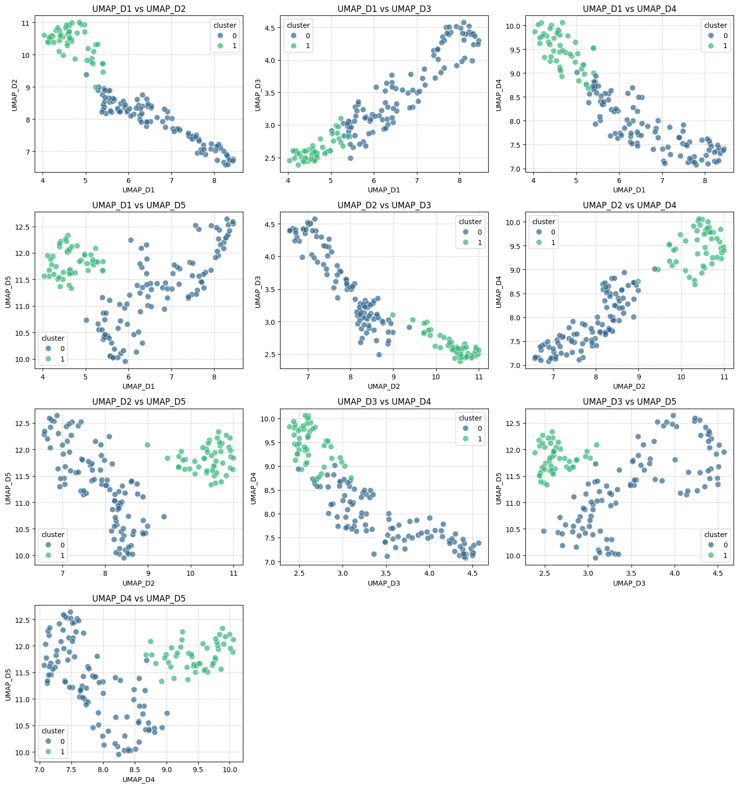
By attempting totally different configurations for HDBSCAN, you might come throughout outcomes by which the variety of recognized clusters could possibly be totally different from two. Simply give it a attempt!
Wrapping Up
As soon as we’ve got gone by way of the method of constructing the text-based clustering pipeline, it’s price concluding by stating the important thing explanation why placing collectively LLM embeddings with HDBSCAN is price it. These embody the flexibility to retain and seize, to some extent, the true semantic which means and linguistic nuances of the unique textual content, due to the properties inherent to embeddings obtained by way of sentence-transformers. Furthermore, HDBSCAN mechanically determines an optimum variety of clusters and is ready to detect outlying factors that may be noise or outliers that might distort group-level statistics.
On this article, you’ll discover ways to construct a textual content clustering pipeline by combining giant language mannequin embeddings with HDBSCAN, a density-based clustering algorithm, to mechanically uncover subjects in unlabeled textual content knowledge.
Matters we’ll cowl embody:
- Learn how to generate textual content embeddings for uncooked paperwork utilizing a pre-trained sentence-transformers mannequin.
- Learn how to cut back the dimensionality of these embeddings with UMAP to arrange them for clustering.
- Learn how to apply HDBSCAN to mechanically uncover matter clusters and visualize the outcomes.
Clustering Unstructured Textual content with LLM Embeddings and HDBSCAN
Introduction
The present period of Generative AI appears to primarily concentrate on chat interfaces and prompts, however the vary of functions of giant language fashions, or LLMs for brief, shouldn’t be restricted to only that. Certainly, one among their strongest downstream talents consists of turning uncooked, messy, unstructured textual content into semantically wealthy mathematical representations known as embeddings. As soon as that’s achieved, we are able to use these textual content representations for quite a lot of machine studying use circumstances, with clustering being no exception.
Particularly, embeddings could be mixed with superior, density-based clustering methods like HDBSCAN, permitting because of this for the invention of hidden subjects, patterns, or classes in your assortment of textual content paperwork: all with out the necessity for prior labeling.
This text reveals tips on how to assemble a text-based clustering pipeline from scratch. We are going to use a freely accessible dataset containing textual content situations, in addition to an open-source LLM that has been skilled for producing embeddings — i.e. a so-called embedding mannequin. The icing on the cake: we’ll use free and useful, fashionable Python libraries offering implementations of clustering algorithms like HDBSCAN.
Step-by-Step Walkthrough
First, let’s begin by putting in the important thing Python libraries we’ll want:
- Sentence transformers, to load a pre-trained LLM for embedding technology from Hugging Face — you’ll want a Hugging Face API key, additionally known as an entry token, to have the ability to load the mannequin.
- Umap-learn, to use an algorithm to scale back the dimensionality of embeddings.
Likewise, if you’re engaged on an area IDE as a substitute of a cloud pocket book setting and don’t have scikit-learn and pandas, you might want to put in them too.
|
!pip set up sentence–transformers umap–be taught |
Now we begin the coding half by getting some contemporary knowledge. The fetch_20newsgroups operate, which fetches a dataset containing texts from categorized information articles, will do. Notice that despite the fact that the dataset accommodates labels, we’ll omit them, as we’re pretending to not know this data for the sake of clustering these knowledge situations into teams primarily based on similarity. Additionally, we pattern down the dataset to 150 situations, which can be consultant sufficient for our instance.
|
import pandas as pd from sklearn.datasets import fetch_20newsgroups
# Fetching a extremely focused subset of information (~150-200 docs) classes = [‘sci.space’, ‘sci.med’, ‘rec.autos’] newsgroups = fetch_20newsgroups(subset=‘practice’, classes=classes, take away=(‘headers’, ‘footers’, ‘quotes’))
# Sampling down right into a consultant, illustrative subset df = pd.DataFrame({‘textual content’: newsgroups.knowledge, ‘true_label’: newsgroups.goal}) df = df[df[‘text’].str.strip().str.len() > 100].pattern(150, random_state=42).reset_index(drop=True)
print(f“Loaded {len(df)} textual content paperwork.”) print(“nSample doc:”) print(df[‘text’].iloc[0][:150] + “…”) |
Output:
|
Loaded 150 textual content paperwork.
Pattern doc:
Okay Mr. Dyer, we‘re correctly impressed along with your philosophical expertise and potential to insult individuals. You’re a fantastic speaker and an adept politic... |
The subsequent step is to acquire the embeddings from uncooked texts. To do that, we load all-MiniLM-L6-v2 from Hugging Face’s sentence-transformers library. This can be a light-weight but efficient mannequin to acquire embeddings shortly.
|
from sentence_transformers import SentenceTransformer
# Loading the free, open-source mannequin mannequin = SentenceTransformer(‘all-MiniLM-L6-v2’)
# Encoding textual content paperwork into dense vector embeddings print(“Producing embeddings…”) embeddings = mannequin.encode(df[‘text’].tolist(), show_progress_bar=True)
print(f“Embedding matrix form: {embeddings.form}”) |
For the reason that embedding dimension is initially too excessive for clustering functions, we now apply a dimensionality discount method through the use of the UMAP algorithm from the namesake library put in earlier:
|
import umap
# Lowering embedding dimensions to five, to retain sufficient density data for clustering reducer = umap.UMAP(n_neighbors=15, n_components=5, min_dist=0.0, random_state=42) reduced_embeddings = reducer.fit_transform(embeddings)
print(f“Lowered matrix form: {reduced_embeddings.form}”) |
Now our numerical embedding vectors related to information articles consist of 5 dimensions (attributes) solely. Let’s see if this compact illustration is significant sufficient to acquire insightful clustering by making use of the HDBSCAN algorithm, which is a density-based clustering strategy:
|
from sklearn.cluster import HDBSCAN
# Initializing HDBSCAN # min_cluster_size=8: we specified that every cluster will need to have no less than 8 paperwork clusterer = HDBSCAN(min_cluster_size=8, min_samples=3, store_centers=‘centroid’) df[‘cluster’] = clusterer.fit_predict(reduced_embeddings)
# Counting situations per cluster cluster_counts = df[‘cluster’].value_counts() print(“nCluster Distribution:”) print(cluster_counts) |
Essential: the clustering outcomes are partly influenced by the hyperparameter settings we outlined for HDBSCAN. I like to recommend you check out different configurations for the minimal cluster measurement and different hyperparameters to discover how this impacts outcomes.
End result:
|
Cluster Distribution: cluster 0 101 1 49 Title: rely, dtype: int64 |
It appears like HDBSCAN detected two clusters related to high-density areas within the knowledge house. Would there even be noisy factors that weren’t allotted to both of those two clusters? Let’s test:
|
for cluster_id in sorted(df[‘cluster’].distinctive()): if cluster_id == –1: print(“n=== CLUSTER: NOISE / UNCLASSIFIED ===”) else: print(f“n=== CLUSTER: Found Subject #{cluster_id} ===”)
# Getting as much as 3 pattern texts from this cluster samples = df[df[‘cluster’] == cluster_id][‘text’].head(3).tolist() for i, pattern in enumerate(samples, 1): clean_sample = ” “.be a part of(pattern.cut up())[:120] print(f” {i}. {clean_sample}…”) |
Output:
|
=== CLUSTER: Found Subject #0 === 1. Okay Mr. Dyer, we‘re correctly impressed along with your philosophical expertise and skill to insult individuals. You’re a fantastic ... 2. I was at an fascinating seminar at work (UK‘s R.A.L. House Science Dept.) on this topic, particularly on a small-scale… 3. That is the second put up which appears to be blurring the excellence between actual illness attributable to Candida albicans and t…
=== CLUSTER: Found Subject #1 === 1. It’s nice that all these different vehicles can out–deal with, out–nook, and out– speed up an Integra. However, you‘ve bought to ask ... 2. l diamond star vehicles (Talon/Eclipse/Laser) put out 190 hp in the turbo fashions, and 195 hp in the AWD turbo fashions, These ... 3. Sorry for the mis–spelling, however I forgot how to spell it after my collection of exams and NO–on hand reference right here. Is it s... |
Looks like all knowledge factors within the pattern of 150 had been allotted to both one of many two clusters recognized, thus hinting on the clue that the information articles would possibly simply separable in line with matter.
For further perception, we are able to present some cluster visualizations with the help of the supplementary code offered under, which reveals a scatterplot for each pairwise mixture of the 5 present parts that describe every knowledge level:
|
1 2 3 4 5 6 7 8 9 10 11 12 13 14 15 16 17 18 19 20 21 22 23 24 25 26 27 28 29 30 31 32 33 34 35 36 |
import matplotlib.pyplot as plt import seaborn as sns import itertools
# Making a DataFrame for the 5 decreased embeddings and cluster labels reduced_df = pd.DataFrame(reduced_embeddings, columns=[f‘UMAP_D{i+1}’ for i in range(reduced_embeddings.shape[1])]) reduced_df[‘cluster’] = df[‘cluster’]
# Getting all distinctive pairwise mixtures of the 5 dimensions dim_pairs = checklist(itertools.mixtures(reduced_df.columns[:–1], 2))
num_plots = len(dim_pairs) num_cols = 3 num_rows = (num_plots + num_cols – 1) // num_cols
plt.determine(figsize=(num_cols * 5, num_rows * 4))
for i, (dim1, dim2) in enumerate(dim_pairs): plt.subplot(num_rows, num_cols, i + 1) sns.scatterplot( x=dim1, y=dim2, hue=‘cluster’, knowledge=reduced_df, palette=‘viridis’, s=70, alpha=0.7, legend=‘full’ ) plt.title(f‘{dim1} vs {dim2}’) plt.xlabel(dim1) plt.ylabel(dim2) plt.grid(True, linestyle=‘–‘, alpha=0.6)
plt.tight_layout() plt.present() |
End result:
By attempting totally different configurations for HDBSCAN, you might come throughout outcomes by which the variety of recognized clusters could possibly be totally different from two. Simply give it a attempt!
Wrapping Up
As soon as we’ve got gone by way of the method of constructing the text-based clustering pipeline, it’s price concluding by stating the important thing explanation why placing collectively LLM embeddings with HDBSCAN is price it. These embody the flexibility to retain and seize, to some extent, the true semantic which means and linguistic nuances of the unique textual content, due to the properties inherent to embeddings obtained by way of sentence-transformers. Furthermore, HDBSCAN mechanically determines an optimum variety of clusters and is ready to detect outlying factors that may be noise or outliers that might distort group-level statistics.


