


Need to know what attracts me to soundscape evaluation?
It’s a discipline that mixes science, creativity, and exploration in a method few others do. To begin with, your laboratory is wherever your toes take you — a forest path, a metropolis park, or a distant mountain path can all develop into areas for scientific discovery and acoustic investigation. Secondly, monitoring a selected geographic space is all about creativity. Innovation is on the coronary heart of environmental audio analysis, whether or not it’s rigging up a customized machine, hiding sensors in tree canopies, or utilizing solar energy for off-grid setups. Lastly, the sheer quantity of knowledge is actually unbelievable, and as we all know, in spatial evaluation, all strategies are truthful sport. From hours of animal calls to the refined hum of city equipment, the acoustic information collected could be huge and complicated, and that opens the door to utilizing every thing from deep studying to geographical info methods (GIS) in making sense of all of it.
After my earlier adventures with soundscape evaluation of one in all Poland’s rivers, I made a decision to lift the bar and design and implement an answer able to analysing soundscapes in actual time. On this weblog put up, you’ll discover a description of the proposed methodology, together with some code that powers your complete course of, primarily utilizing an Audio Spectrogram Transformer (AST) for sound classification.

Strategies
Setup
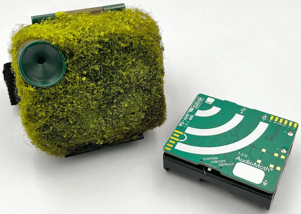
There are numerous the reason why, on this explicit case, I selected to make use of a mixture of Raspberry Pi 4 and AudioMoth. Consider me, I examined a variety of gadgets — from much less power-hungry fashions of the Raspberry Pi household, by varied Arduino variations, together with the Portenta, all the way in which to the Jetson Nano. And that was only the start. Selecting the best microphone turned out to be much more sophisticated.
In the end, I went with the Pi 4 B (4GB RAM) due to its strong efficiency and comparatively low energy consumption (~700mAh when operating my code). Moreover, pairing it with the AudioMoth in USB microphone mode gave me a number of flexibility throughout prototyping. AudioMoth is a strong machine with a wealth of configuration choices, e.g. sampling charge from 8 kHz to beautiful 384 kHz. I’ve a powerful feeling that — in the long term — it will show to be an ideal alternative for my soundscape research.

Capturing sound
Capturing audio from a USB microphone utilizing Python turned out to be surprisingly troublesome. After battling varied libraries for some time, I made a decision to fall again on the great previous Linux arecord. The entire sound seize mechanism is encapsulated with the next command:
arecord -d 1 -D plughw:0,7 -f S16_LE -r 16000 -c 1 -q /tmp/audio.wavI’m intentionally utilizing a plug-in machine to allow automated conversion in case I want to introduce any modifications to the USB microphone configuration. AST is run on 16 kHz samples, so the recording and AudioMoth sampling are set to this worth.
Take note of the generator within the code. It’s vital that the machine repeatedly captures audio on the time intervals I specify. I aimed to retailer solely the newest audio pattern on the machine and discard it after the classification. This strategy will probably be particularly helpful later throughout larger-scale research in city areas, because it helps guarantee folks’s privateness and aligns with GDPR compliance.
import asyncio
import re
import subprocess
from tempfile import TemporaryDirectory
from typing import Any, AsyncGenerator

import librosa
import numpy as np


class AudioDevice:
    def __init__(
        self,
        title: str,
        channels: int,
        sampling_rate: int,
        format: str,
    ):
        self.title = self._match_device(title)
        self.channels = channels
        self.sampling_rate = sampling_rate
        self.format = format

    @staticmethod
    def _match_device(title: str):
        traces = subprocess.check_output(['arecord', '-l'], textual content=True).splitlines()
        gadgets = [
            f'plughw:{m.group(1)},{m.group(2)}'
            for line in lines
            if name.lower() in line.lower()
            if (m := re.search(r'card (d+):.*device (d+):', line))
        ]

        if len(gadgets) == 0:
            increase ValueError(f'No gadgets discovered matching `{title}`')
        if len(gadgets) > 1:
            increase ValueError(f'A number of gadgets discovered matching `{title}` -> {gadgets}')
        return gadgets[0]

    async def continuous_capture(
        self,
        sample_duration: int = 1,
        capture_delay: int = 0,
    ) -> AsyncGenerator[np.ndarray, Any]:
        with TemporaryDirectory() as temp_dir:
            temp_file = f'{temp_dir}/audio.wav'
            command = (
                f'arecord '
                f'-d {sample_duration} '
                f'-D {self.title} '
                f'-f {self.format} '
                f'-r {self.sampling_rate} '
                f'-c {self.channels} '
                f'-q '
                f'{temp_file}'
            )

            whereas True:
                subprocess.check_call(command, shell=True)
                information, sr = librosa.load(
                    temp_file,
                    sr=self.sampling_rate,
                )
                await asyncio.sleep(capture_delay)
                yield information
Classification
Now for essentially the most thrilling half.
Utilizing the Audio Spectrogram Transformer (AST) and the wonderful HuggingFace ecosystem, we are able to effectively analyse audio and classify detected segments into over 500 classes.
Word that I’ve ready the system to help varied pre-trained fashions. By default, I exploit MIT/ast-finetuned-audioset-10–10–0.4593, because it delivers one of the best outcomes and runs properly on the Raspberry Pi 4. Nonetheless, onnx-community/ast-finetuned-audioset-10–10–0.4593-ONNX can be price exploring — particularly its quantised model, which requires much less reminiscence and serves the inference outcomes faster.
Chances are you’ll discover that I’m not limiting the mannequin to a single classification label, and that’s intentional. As a substitute of assuming that just one sound supply is current at any given time, I apply a sigmoid operate to the mannequin’s logits to acquire impartial chances for every class. This enables the mannequin to specific confidence in a number of labels concurrently, which is essential for real-world soundscapes the place overlapping sources — like birds, wind, and distant visitors — typically happen collectively. Taking the prime 5 outcomes ensures that the system captures the more than likely sound occasions within the pattern with out forcing a winner-takes-all resolution.
from pathlib import Path
from typing import Non-obligatory

import numpy as np
import pandas as pd
import torch
from optimum.onnxruntime import ORTModelForAudioClassification
from transformers import AutoFeatureExtractor, ASTForAudioClassification


class AudioClassifier:
    def __init__(self, pretrained_ast: str, pretrained_ast_file_name: Non-obligatory[str] = None):
        if pretrained_ast_file_name and Path(pretrained_ast_file_name).suffix == '.onnx':
            self.mannequin = ORTModelForAudioClassification.from_pretrained(
                pretrained_ast,
                subfolder='onnx',
                file_name=pretrained_ast_file_name,
            )
            self.feature_extractor = AutoFeatureExtractor.from_pretrained(
                pretrained_ast,
                file_name=pretrained_ast_file_name,
            )
        else:
            self.mannequin = ASTForAudioClassification.from_pretrained(pretrained_ast)
            self.feature_extractor = AutoFeatureExtractor.from_pretrained(pretrained_ast)

        self.sampling_rate = self.feature_extractor.sampling_rate

    async def predict(
        self,
        audio: np.array,
        top_k: int = 5,
    ) -> pd.DataFrame:
        with torch.no_grad():
            inputs = self.feature_extractor(
                audio,
                sampling_rate=self.sampling_rate,
                return_tensors='pt',
            )
            logits = self.mannequin(**inputs).logits[0]
            proba = torch.sigmoid(logits)
            top_k_indices = torch.argsort(proba)[-top_k:].flip(dims=(0,)).tolist()

            return pd.DataFrame(
                {
                    'label': [self.model.config.id2label[i] for i in top_k_indices],
                    'rating': proba[top_k_indices],
                }
            )
To run the ONNX model of the mannequin, it is advisable add Optimum to your dependencies.
Sound strain degree
Together with the audio classification, I seize info on sound strain degree. This strategy not solely identifies what made the sound but additionally positive factors perception into how strongly every sound was current. In that method, the mannequin captures a richer, extra sensible illustration of the acoustic scene and might ultimately be used to detect finer-grained noise air pollution info.
import numpy as np
from maad.spl import wav2dBSPL
from maad.util import mean_dB


async def calculate_sound_pressure_level(audio: np.ndarray, acquire=10 + 15, sensitivity=-18) -> np.ndarray:
    x = wav2dBSPL(audio, acquire=acquire, sensitivity=sensitivity, Vadc=1.25)
    return mean_dB(x, axis=0)
The acquire (preamp + amp), sensitivity (dB/V), and Vadc (V) are set primarily for AudioMoth and confirmed experimentally. In case you are utilizing a distinct machine, you should determine these values by referring to the technical specification.
Storage
Knowledge from every sensor is synchronised with a PostgreSQL database each 30 seconds. The present city soundscape monitor prototype makes use of an Ethernet connection; subsequently, I’m not restricted when it comes to community load. The machine for extra distant areas will synchronise the information every hour utilizing a GSM connection.
label           rating        machine   sync_id                                sync_time
Hum             0.43894055   yor      9531b89a-4b38-4a43-946b-43ae2f704961   2025-05-26 14:57:49.104271
Mains hum       0.3894045    yor      9531b89a-4b38-4a43-946b-43ae2f704961   2025-05-26 14:57:49.104271
Static          0.06389702   yor      9531b89a-4b38-4a43-946b-43ae2f704961   2025-05-26 14:57:49.104271
Buzz            0.047603738  yor      9531b89a-4b38-4a43-946b-43ae2f704961   2025-05-26 14:57:49.104271
White noise     0.03204195   yor      9531b89a-4b38-4a43-946b-43ae2f704961   2025-05-26 14:57:49.104271
Bee, wasp, and so on. 0.40881288   yor      8477e05c-0b52-41b2-b5e9-727a01b9ec87   2025-05-26 14:58:40.641071
Fly, housefly   0.38868183   yor      8477e05c-0b52-41b2-b5e9-727a01b9ec87   2025-05-26 14:58:40.641071
Insect          0.35616025   yor      8477e05c-0b52-41b2-b5e9-727a01b9ec87   2025-05-26 14:58:40.641071
Speech          0.23579548   yor      8477e05c-0b52-41b2-b5e9-727a01b9ec87   2025-05-26 14:58:40.641071
Buzz            0.105577625  yor      8477e05c-0b52-41b2-b5e9-727a01b9ec87   2025-05-26 14:58:40.641071
Outcomes
A separate software, constructed utilizing Streamlit and Plotly, accesses this information. At present, it shows details about the machine’s location, temporal SPL (sound strain degree), recognized sound lessons, and a spread of acoustic indices.

And now we’re good to go. The plan is to increase the sensor community and attain round 20 gadgets scattered round a number of locations in my metropolis. Extra details about a bigger space sensor deployment will probably be out there quickly.
Furthermore, I’m gathering information from a deployed sensor and plan to share the information bundle, dashboard, and evaluation in an upcoming weblog put up. I’ll use an attention-grabbing strategy that warrants a deeper dive into audio classification. The principle thought is to match totally different sound strain ranges to the detected audio lessons. I hope to discover a higher method of describing noise air pollution. So keep tuned for a extra detailed breakdown quickly.
Within the meantime, you possibly can learn the preliminary paper on my soundscapes research (headphones are compulsory).
This put up was proofread and edited utilizing Grammarly to enhance grammar and readability.


