


is co-authored by Felipe Bandeira, Giselle Fretta, Thu Than, and Elbion Redenica. We additionally thank Prof. Carl Scheffler for his assist.
Introduction
Parameter estimation has been for many years one of the vital necessary matters in statistics. Whereas frequentist approaches, equivalent to Most Probability Estimations, was the gold commonplace, the advance of computation has opened house for Bayesian strategies. Estimating posterior distributions with Mcmc samplers grew to become more and more frequent, however dependable inferences rely upon a job that’s removed from trivial: ensuring that the sampler — and the processes it executes beneath the hood — labored as anticipated. Holding in thoughts what Lewis Caroll as soon as wrote: “For those who don’t know the place you’re going, any highway will take you there.”
This text is supposed to assist information scientists consider an usually ignored facet of Bayesian parameter estimation: the reliability of the sampling course of. All through the sections, we mix easy analogies with technical rigor to make sure our explanations are accessible to information scientists with any stage of familiarity with Bayesian strategies. Though our implementations are in Python with PyMC, the ideas we cowl are helpful to anybody utilizing an MCMC algorithm, from Metropolis-Hastings to NUTS.
Key Ideas
No information scientist or statistician would disagree with the significance of strong parameter estimation strategies. Whether or not the target is to make inferences or conduct simulations, having the capability to mannequin the information era course of is a vital a part of the method. For a very long time, the estimations had been primarily carried out utilizing frequentist instruments, equivalent to Most Probability Estimations (MLE) and even the well-known Least Squares optimization utilized in regressions. But, frequentist strategies have clear shortcomings, equivalent to the truth that they’re targeted on level estimates and don’t incorporate prior information that would enhance estimates.
As a substitute for these instruments, Bayesian strategies have gained recognition over the previous a long time. They supply statisticians not solely with level estimates of the unknown parameter but in addition with confidence intervals for it, all of that are knowledgeable by the information and by the prior information researchers held. Initially, Bayesian parameter estimation was completed by way of an tailored model of Bayes’ theorem targeted on unknown parameters (represented as θ) and identified information factors (represented as x). We will outline P(θ|x), the posterior distribution of a parameter’s worth given the information, as:
[ P(theta|x) = fractheta) P(theta){P(x)} ]
On this formulation, P(x|θ) is the probability of the information given a parameter worth, P(θ) is the prior distribution over the parameter, and P(x) is the proof, which is computed by integrating all potential values of the prior:
[ P(x) = int_theta P(x, theta) dtheta ]
In some circumstances, because of the complexity of the calculations required, deriving the posterior distribution analytically was not potential. Nevertheless, with the advance of computation, operating sampling algorithms (particularly MCMC ones) to estimate posterior distributions has change into simpler, giving researchers a robust device for conditions the place analytical posteriors are usually not trivial to seek out. But, with such energy additionally comes a considerable amount of accountability to make sure that outcomes make sense. That is the place sampler diagnostics are available, providing a set of helpful instruments to gauge 1) whether or not an MCMC algorithm is working properly and, consequently, 2) whether or not the estimated distribution we see is an correct illustration of the actual posterior distribution. However how can we all know so?
How samplers work
Earlier than diving into the technicalities of diagnostics, we will cowl how the method of sampling a posterior (particularly with an MCMC sampler) works. In easy phrases, we will consider a posterior distribution as a geographical space we haven’t been to however have to know the topography of. How can we draw an correct map of the area?
Considered one of our favourite analogies comes from Ben Gilbert. Suppose that the unknown area is definitely a home whose floorplan we want to map. For some purpose, we can not instantly go to the home, however we will ship bees inside with GPS gadgets hooked up to them. If the whole lot works as anticipated, the bees will fly round the home, and utilizing their trajectories, we will estimate what the ground plan seems like. On this analogy, the ground plan is the posterior distribution, and the sampler is the group of bees flying round the home.
The rationale we’re writing this text is that, in some circumstances, the bees gained’t fly as anticipated. In the event that they get caught in a sure room for some purpose (as a result of somebody dropped sugar on the ground, for instance), the information they return gained’t be consultant of all the home; somewhat than visiting all rooms, the bees solely visited a number of, and our image of what the home seems like will in the end be incomplete. Equally, when a sampler doesn’t work accurately, our estimation of the posterior distribution can be incomplete, and any inference we draw primarily based on it’s prone to be fallacious.
Monte Carlo Markov Chain (MCMC)
In technical phrases, we name an MCMC course of any algorithm that undergoes transitions from one state to a different with sure properties. Markov Chain refers to the truth that the following state solely depends upon the present one (or that the bee’s subsequent location is just influenced by its present place, and never by all the locations the place it has been earlier than). Monte Carlo implies that the following state is chosen randomly. MCMC strategies like Metropolis-Hastings, Gibbs sampling, Hamiltonian Monte Carlo (HMC), and No-U-Flip Sampler (NUTS) all function by establishing Markov Chains (a sequence of steps) which are near random and step by step discover the posterior distribution.
Now that you simply perceive how a sampler works, let’s dive right into a sensible situation to assist us discover sampling issues.
Case Examine
Think about that, in a faraway nation, a governor needs to grasp extra about public annual spending on healthcare by mayors of cities with lower than 1 million inhabitants. Reasonably than taking a look at sheer frequencies, he needs to grasp the underlying distribution explaining expenditure, and a pattern of spending information is about to reach. The issue is that two of the economists concerned within the undertaking disagree about how the mannequin ought to look.
Mannequin 1
The primary economist believes that every one cities spend equally, with some variation round a sure imply. As such, he creates a easy mannequin. Though the specifics of how the economist selected his priors are irrelevant to us, we do have to needless to say he’s making an attempt to approximate a Regular (unimodal) distribution.
[
x_i sim text{Normal}(mu, sigma^2) text{ i.i.d. for all } i
mu sim text{Normal}(10, 2)
sigma^2 sim text{Uniform}(0,5)
]
Mannequin 2
The second economist disagrees, arguing that spending is extra complicated than his colleague believes. He believes that, given ideological variations and funds constraints, there are two sorts of cities: those that do their finest to spend little or no and those that aren’t afraid of spending loads. As such, he creates a barely extra complicated mannequin, utilizing a mix of normals to replicate his perception that the true distribution is bimodal.
[
x_i sim text{Normal-Mixture}([omega, 1-omega], [m_1, m_2], [s_1^2, s_2^2]) textual content{ i.i.d. for all } i
m_j sim textual content{Regular}(2.3, 0.5^2) textual content{ for } j = 1,2
s_j^2 sim textual content{Inverse-Gamma}(1,1) textual content{ for } j=1,2
omega sim textual content{Beta}(1,1)
]
After the information arrives, every economist runs an MCMC algorithm to estimate their desired posteriors, which shall be a mirrored image of actuality (1) if their assumptions are true and (2) if the sampler labored accurately. The primary if, a dialogue about assumptions, shall be left to the economists. Nevertheless, how can they know whether or not the second if holds? In different phrases, how can they ensure that the sampler labored accurately and, as a consequence, their posterior estimations are unbiased?
Sampler Diagnostics
To guage a sampler’s efficiency, we will discover a small set of metrics that replicate totally different components of the estimation course of.
Quantitative Metrics
R-hat (Potential Scale Discount Issue)
In easy phrases, R-hat evaluates whether or not bees that began at totally different locations have all explored the identical rooms on the finish of the day. To estimate the posterior, an MCMC algorithm makes use of a number of chains (or bees) that begin at random places. R-hat is the metric we use to evaluate the convergence of the chains. It measures whether or not a number of MCMC chains have combined properly (i.e., if they’ve sampled the identical topography) by evaluating the variance of samples inside every chain to the variance of the pattern means throughout chains. Intuitively, which means that
[
hat{R} = sqrt{frac{text{Variance Between Chains}}{text{Variance Within Chains}}}
]
If R-hat is near 1.0 (or under 1.01), it implies that the variance inside every chain is similar to the variance between chains, suggesting that they’ve converged to the identical distribution. In different phrases, the chains are behaving equally and are additionally indistinguishable from each other. That is exactly what we see after sampling the posterior of the primary mannequin, proven within the final column of the desk under:

The r-hat from the second mannequin, nonetheless, tells a unique story. The very fact we now have such massive r-hat values signifies that, on the finish of the sampling course of, the totally different chains had not converged but. In follow, which means that the distribution they explored and returned was totally different, or that every bee created a map of a unique room of the home. This basically leaves us with no clue of how the items join or what the whole flooring plan seems like.

Given our R-hat readouts had been massive, we all know one thing went fallacious with the sampling course of within the second mannequin. Nevertheless, even when the R-hat had turned out inside acceptable ranges, this doesn’t give us certainty that the sampling course of labored. R-hat is only a diagnostic device, not a assure. Typically, even when your R-hat readout is decrease than 1.01, the sampler may not have correctly explored the complete posterior. This occurs when a number of bees begin their exploration in the identical room and stay there. Likewise, for those who’re utilizing a small variety of chains, and in case your posterior occurs to be multimodal, there’s a chance that every one chains began in the identical mode and didn’t discover different peaks.
The R-hat readout displays convergence, not completion. So as to have a extra complete thought, we have to examine different diagnostic metrics as properly.
Efficient Pattern Dimension (ESS)
When explaining what MCMC was, we talked about that “Monte Carlo” refers to the truth that the following state is chosen randomly. This doesn’t essentially imply that the states are totally impartial. Although the bees select their subsequent step at random, these steps are nonetheless correlated to some extent. If a bee is exploring a lounge at time t=0, it’s going to most likely nonetheless be in the lounge at time t=1, despite the fact that it’s in a unique a part of the identical room. As a consequence of this pure connection between samples, we are saying these two information factors are autocorrelated.
As a consequence of their nature, MCMC strategies inherently produce autocorrelated samples, which complicates statistical evaluation and requires cautious analysis. In statistical inference, we frequently assume impartial samples to make sure that the estimates of uncertainty are correct, therefore the necessity for uncorrelated samples. If two information factors are too related to one another, the correlation reduces their efficient data content material. Mathematically, the formulation under represents the autocorrelation operate between two time factors (t1 and t2) in a random course of:
[
R_{XX}(t_1, t_2) = E[X_{t_1} overline{X_{t_2}}]
]
the place E is the anticipated worth operator and X-bar is the complicated conjugate. In MCMC sampling, that is essential as a result of excessive autocorrelation implies that new samples don’t educate us something totally different from the previous ones, successfully decreasing the pattern dimension we now have. Unsurprisingly, the metric that displays that is known as Efficient Pattern Dimension (ESS), and it helps us decide what number of actually impartial samples we now have.
As hinted beforehand, the efficient pattern dimension accounts for autocorrelation by estimating what number of actually impartial samples would offer the identical data because the autocorrelated samples we now have. Mathematically, for a parameter θ, the ESS is outlined as:
[
ESS = frac{n}{1 + 2 sum_{k=1}^{infty} rho(theta)_k}
]
the place n is the full variety of samples and ρ(θ)ok is the autocorrelation at lag ok for parameter θ.
Sometimes, for ESS readouts, the upper, the higher. That is what we see within the readout for the primary mannequin. Two frequent ESS variations are Bulk-ESS, which assesses mixing within the central a part of the distribution, and Tail-ESS, which focuses on the effectivity of sampling the distribution’s tails. Each inform us if our mannequin precisely displays the central tendency and credible intervals.

In distinction, the readouts for the second mannequin are very dangerous. Sometimes, we wish to see readouts which are at the least 1/10 of the full pattern dimension. On this case, given every chain sampled 2000 observations, we should always count on ESS readouts of at the least 800 (from the full dimension of 8000 samples throughout 4 chains of 2000 samples every), which isn’t what we observe.

Visible Diagnostics
Aside from the numerical metrics, our understanding of sampler efficiency may be deepened by way of the usage of diagnostic plots. The principle ones are rank plots, hint plots, and pair plots.
Rank Plots
A rank plot helps us determine whether or not the totally different chains have explored all the posterior distribution. If we as soon as once more consider the bee analogy, rank plots inform us which bees explored which components of the home. Due to this fact, to guage whether or not the posterior was explored equally by all chains, we observe the form of the rank plots produced by the sampler. Ideally, we would like the distribution of all chains to look roughly uniform, like within the rank plots generated after sampling the primary mannequin. Every coloration under represents a series (or bee):
Below the hood, a rank plot is produced with a easy sequence of steps. First, we run the sampler and let it pattern from the posterior of every parameter. In our case, we’re sampling posteriors for parameters m and s of the primary mannequin. Then, parameter by parameter, we get all samples from all chains, put them collectively, and organize them from smallest to largest. We then ask ourselves, for every pattern, what was the chain the place it got here from? It will enable us to create plots like those we see above.
In distinction, dangerous rank plots are simple to identify. In contrast to the earlier instance, the distributions from the second mannequin, proven under, are usually not uniform. From the plots, what we interpret is that every chain, after starting at totally different random places, acquired caught in a area and didn’t discover everything of the posterior. Consequently, we can not make inferences from the outcomes, as they’re unreliable and never consultant of the true posterior distribution. This is able to be equal to having 4 bees that began at totally different rooms of the home and acquired caught someplace throughout their exploration, by no means overlaying everything of the property.
KDE and Hint Plots
Much like R-hat, hint plots assist us assess the convergence of MCMC samples by visualizing how the algorithm explores the parameter house over time. PyMC offers two kinds of hint plots to diagnose mixing points: Kernel Density Estimate (KDE) plots and iteration-based hint plots. Every of those serves a definite goal in evaluating whether or not the sampler has correctly explored the goal distribution.
The KDE plot (normally on the left) estimates the posterior density for every chain, the place every line represents a separate chain. This enables us to examine whether or not all chains have converged to the identical distribution. If the KDEs overlap, it means that the chains are sampling from the identical posterior and that mixing has occurred. Then again, the hint plot (normally on the best) visualizes how parameter values change over MCMC iterations (steps), with every line representing a unique chain. A well-mixed sampler will produce hint plots that look noisy and random, with no clear construction or separation between chains.
Utilizing the bee analogy, hint plots may be regarded as snapshots of the “options” of the home at totally different places. If the sampler is working accurately, the KDEs within the left plot ought to align carefully, exhibiting that every one bees (chains) have explored the home equally. In the meantime, the best plot ought to present extremely variable traces that mix collectively, confirming that the chains are actively transferring by way of the house somewhat than getting caught in particular areas.

Nevertheless, in case your sampler has poor mixing or convergence points, you will notice one thing just like the determine under. On this case, the KDEs is not going to overlap, that means that totally different chains have sampled from totally different distributions somewhat than a shared posterior. The hint plot may also present structured patterns as a substitute of random noise, indicating that chains are caught in numerous areas of the parameter house and failing to totally discover it.

By utilizing hint plots alongside the opposite diagnostics, you may determine sampling points and decide whether or not your MCMC algorithm is successfully exploring the posterior distribution.
Pair Plots
A 3rd form of plot that’s usually helpful for diagnostic are pair plots. In fashions the place we wish to estimate the posterior distribution of a number of parameters, pair plots enable us to look at how totally different parameters are correlated. To know how such plots are fashioned, assume once more concerning the bee analogy. For those who think about that we’ll create a plot with the width and size of the home, every “step” that the bees take may be represented by an (x, y) mixture. Likewise, every parameter of the posterior is represented as a dimension, and we create scatter plots exhibiting the place the sampler walked utilizing parameter values as coordinates. Right here, we’re plotting every distinctive pair (x, y), ensuing within the scatter plot you see in the course of the picture under. The one-dimensional plots you see on the perimeters are the marginal distributions over every parameter, giving us extra data on the sampler’s habits when exploring them.
Check out the pair plot from the primary mannequin.

Every axis represents one of many two parameters whose posteriors we’re estimating. For now, let’s concentrate on the scatter plot within the center, which reveals the parameter mixtures sampled from the posterior. The very fact we now have a really even distribution implies that, for any explicit worth of m, there was a variety of values of s that had been equally prone to be sampled. Moreover, we don’t see any correlation between the 2 parameters, which is normally good! There are circumstances after we would count on some correlation, equivalent to when our mannequin includes a regression line. Nevertheless, on this occasion, we now have no purpose to imagine two parameters ought to be extremely correlated, so the actual fact we don’t observe uncommon habits is constructive information.
Now, check out the pair plots from the second mannequin.

On condition that this mannequin has 5 parameters to be estimated, we naturally have a higher variety of plots since we’re analyzing them pair-wise. Nevertheless, they give the impression of being odd in comparison with the earlier instance. Specifically, somewhat than having a fair distribution of factors, the samples right here both appear to be divided throughout two areas or appear considerably correlated. That is one other method of visualizing what the rank plots have proven: the sampler didn’t discover the complete posterior distribution. Under we remoted the highest left plot, which comprises the samples from m0 and m1. In contrast to the plot from mannequin 1, right here we see that the worth of 1 parameter drastically influences the worth of the opposite. If we sampled m1 round 2.5, for instance, m0 is prone to be sampled from a really slim vary round 1.5.

Sure shapes may be noticed in problematic pair plots comparatively incessantly. Diagonal patterns, for instance, point out a excessive correlation between parameters. Banana shapes are sometimes related to parametrization points, usually being current in fashions with tight priors or constrained parameters. Funnel shapes would possibly point out hierarchical fashions with dangerous geometry. When we now have two separate islands, like within the plot above, this may point out that the posterior is bimodal AND that the chains haven’t combined properly. Nevertheless, needless to say these shapes would possibly point out issues, however not essentially achieve this. It’s as much as the information scientist to look at the mannequin and decide which behaviors are anticipated and which of them are usually not!
Some Fixing Strategies
When your diagnostics point out sampling issues — whether or not regarding R-hat values, low ESS, uncommon rank plots, separated hint plots, or unusual parameter correlations in pair plots — a number of methods might help you tackle the underlying points. Sampling issues sometimes stem from the goal posterior being too complicated for the sampler to discover effectively. Complicated goal distributions might need:
- A number of modes (peaks) that the sampler struggles to maneuver between
- Irregular shapes with slim “corridors” connecting totally different areas
- Areas of drastically totally different scales (just like the “neck” of a funnel)
- Heavy tails which are troublesome to pattern precisely
Within the bee analogy, these complexities symbolize homes with uncommon flooring plans — disconnected rooms, extraordinarily slim hallways, or areas that change dramatically in dimension. Simply as bees would possibly get trapped in particular areas of such homes, MCMC chains can get caught in sure areas of the posterior.


To assist the sampler in its exploration, there are easy methods we will use.
Technique 1: Reparameterization
Reparameterization is especially efficient for hierarchical fashions and distributions with difficult geometries. It includes remodeling your mannequin’s parameters to make them simpler to pattern. Again to the bee analogy, think about the bees are exploring a home with a peculiar format: a spacious lounge that connects to the kitchen by way of a really, very slim hallway. One facet we hadn’t talked about earlier than is that the bees should fly in the identical method by way of all the home. That implies that if we dictate the bees ought to use massive “steps,” they’ll discover the lounge very properly however hit the partitions within the hallway head-on. Likewise, if their steps are small, they’ll discover the slim hallway properly, however take without end to cowl all the lounge. The distinction in scales, which is pure to the home, makes the bees’ job tougher.
A traditional instance that represents this situation is Neal’s funnel, the place the size of 1 parameter depends upon one other:
[
p(y, x) = text{Normal}(y|0, 3) times prod_{n=1}^{9} text{Normal}(x_n|0, e^{y/2})
]

We will see that the size of x relies on the worth of y. To repair this downside, we will separate x and y as impartial commonplace Normals after which remodel these variables into the specified funnel distribution. As an alternative of sampling instantly like this:
[
begin{align*}
y &sim text{Normal}(0, 3)
x &sim text{Normal}(0, e^{y/2})
end{align*}
]
You’ll be able to reparameterize to pattern from commonplace Normals first:
[
y_{raw} sim text{Standard Normal}(0, 1)
x_{raw} sim text{Standard Normal}(0, 1)
y = 3y_{raw}
x = e^{y/2} x_{raw}
]
This system separates the hierarchical parameters and makes sampling extra environment friendly by eliminating the dependency between them.
Reparameterization is like redesigning the home such that as a substitute of forcing the bees to discover a single slim hallway, we create a brand new format the place all passages have related widths. This helps the bees use a constant flying sample all through their exploration.
Technique 2: Dealing with Heavy-tailed Distributions
Heavy-tailed distributions like Cauchy and Pupil-T current challenges for samplers and the perfect step dimension. Their tails require bigger step sizes than their central areas (just like very lengthy hallways that require the bees to journey lengthy distances), which creates a problem:
- Small step sizes result in inefficient sampling within the tails
- Giant step sizes trigger too many rejections within the heart

Reparameterization options embrace:
- For Cauchy: Defining the variable as a metamorphosis of a Uniform distribution utilizing the Cauchy inverse CDF
- For Pupil-T: Utilizing a Gamma-Combination illustration
Technique 3: Hyperparameter Tuning
Typically the answer lies in adjusting the sampler’s hyperparameters:
- Improve whole iterations: The best method — give the sampler extra time to discover.
- Improve goal acceptance fee (adapt_delta): Scale back divergent transitions (strive 0.9 as a substitute of the default 0.8 for complicated fashions, for instance).
- Improve max_treedepth: Permit the sampler to take extra steps per iteration.
- Prolong warmup/adaptation section: Give the sampler extra time to adapt to the posterior geometry.
Keep in mind that whereas these changes could enhance your diagnostic metrics, they usually deal with signs somewhat than underlying causes. The earlier methods (reparameterization and higher proposal distributions) sometimes provide extra basic options.
Technique 4: Higher Proposal Distributions
This answer is for operate becoming processes, somewhat than sampling estimations of the posterior. It mainly asks the query: “I’m at the moment right here on this panorama. The place ought to I soar to subsequent in order that I discover the complete panorama, or how do I do know that the following soar is the soar I ought to make?” Thus, selecting an excellent distribution means ensuring that the sampling course of explores the complete parameter house as a substitute of only a particular area. An excellent proposal distribution ought to:
- Have substantial chance mass the place the goal distribution does.
- Permit the sampler to make jumps of the suitable dimension.
One frequent alternative of the proposal distribution is the Gaussian (Regular) distribution with imply μ and commonplace deviation σ — the size of the distribution that we will tune to determine how far to leap from the present place to the following place. If we select the size for the proposal distribution to be too small, it would both take too lengthy to discover all the posterior or it’s going to get caught in a area and by no means discover the complete distribution. But when the size is simply too massive, you would possibly by no means get to discover some areas, leaping over them. It’s like taking part in ping-pong the place we solely attain the 2 edges however not the center.
Enhance Prior Specification
When all else fails, rethink your mannequin’s prior specs. Obscure or weakly informative priors (like uniformly distributed priors) can typically result in sampling difficulties. Extra informative priors, when justified by area information, might help information the sampler towards extra cheap areas of the parameter house. Typically, regardless of your finest efforts, a mannequin could stay difficult to pattern successfully. In such circumstances, contemplate whether or not a less complicated mannequin would possibly obtain related inferential objectives whereas being extra computationally tractable. The perfect mannequin is usually not probably the most complicated one, however the one which balances complexity with reliability. The desk under reveals the abstract of fixing methods for various points.
| Diagnostic Sign | Potential Situation | Really useful Repair |
| Excessive R-hat | Poor mixing between chains | Improve iterations, alter the step dimension |
| Low ESS | Excessive autocorrelation | Reparameterization, enhance adapt_delta |
| Non-uniform rank plots | Chains caught in numerous areas | Higher proposal distribution, begin with a number of chains |
| Separated KDEs in hint plots | Chains exploring totally different distributions | Reparameterization |
| Funnel shapes in pair plots | Hierarchical mannequin points | Non-centered reparameterization |
| Disjoint clusters in pair plots | Multimodality with poor mixing | Adjusted distribution, simulated annealing |
Conclusion
Assessing the standard of MCMC sampling is essential for making certain dependable inference. On this article, we explored key diagnostic metrics equivalent to R-hat, ESS, rank plots, hint plots, and pair plots, discussing how every helps decide whether or not the sampler is performing correctly.
If there’s one takeaway we would like you to remember it’s that you need to at all times run diagnostics earlier than drawing conclusions out of your samples. No single metric offers a definitive reply — every serves as a device that highlights potential points somewhat than proving convergence. When issues come up, methods equivalent to reparameterization, hyperparameter tuning, and prior specification might help enhance sampling effectivity.
By combining these diagnostics with considerate modeling selections, you may guarantee a extra strong evaluation, decreasing the chance of deceptive inferences because of poor sampling habits.
References
B. Gilbert, Bob’s bees: the significance of utilizing a number of bees (chains) to evaluate MCMC convergence (2018), Youtube
Chi-Feng, MCMC demo (n.d.), GitHub
D. Simpson, Perhaps it’s time to let the previous methods die; or We broke R-hat so now we now have to repair it. (2019), Statistical Modeling, Causal Inference, and Social Science
M. Taboga, Markov Chain Monte Carlo (MCMC) strategies (2021), Lectures on chance principle and mathematical Statistics. Kindle Direct Publishing.
T. Wiecki, MCMC Sampling for Dummies (2024), twecki.io
Stan Person’s Information, Reparametrization (n.d.), Stan Documentation


