


Exploring standard reinforcement studying environments, in a beginner-friendly approach
It is a guided sequence on introductory RL ideas utilizing the environments from the OpenAI Gymnasium Python package deal. This primary article will cowl the high-level ideas mandatory to know and implement Q-learning to unravel the “Frozen Lake” atmosphere.
Completely happy studying ❤ !
Let’s discover reinforcement studying by evaluating it to acquainted examples from on a regular basis life.
Card Sport — Think about taking part in a card sport: Whenever you first be taught the sport, the principles could also be unclear. The playing cards you play may not be probably the most optimum and the methods you employ is perhaps imperfect. As you play extra and possibly win a couple of video games, you be taught what playing cards to play when and what methods are higher than others. Typically it’s higher to bluff, however different occasions it is best to in all probability fold; saving a wild card for later use is perhaps higher than taking part in it instantly. Understanding what the optimum plan of action is discovered by means of a mixture of expertise and reward. Your expertise comes from taking part in the sport and also you get rewarded when your methods work nicely, maybe resulting in a victory or new excessive rating.

Classical Conditioning — By ringing a bell earlier than he fed a canine, Ivan Pavlov demonstrated the connection between exterior stimulus and a physiological response. The canine was conditioned to affiliate the sound of the bell with being fed and thus started to drool on the sound of the bell, even when no meals was current. Although not strictly an instance of reinforcement studying, by means of repeated experiences the place the canine was rewarded with meals on the sound of the bell, it nonetheless discovered to affiliate the 2 collectively.
Suggestions Management — An utility of management idea present in engineering disciplines the place a system’s behaviour might be adjusted by offering suggestions to a controller. As a subset of suggestions management, reinforcement studying requires suggestions from our present atmosphere to affect our actions. By offering suggestions within the type of reward, we will incentivize our agent to choose the optimum course of motion.
The Agent, State, and Atmosphere
Reinforcement studying is a studying course of constructed on the buildup of previous experiences coupled with quantifiable reward. In every instance, we illustrate how our experiences can affect our actions and the way reinforcing a optimistic affiliation between reward and response may probably be used to unravel sure issues. If we will be taught to affiliate reward with an optimum motion, we may derive an algorithm that may choose actions that yield the best possible reward.
In reinforcement studying, the “learner” is known as the agent. The agent interacts with the environment and, by means of its actions, learns what is taken into account “good” or “dangerous” primarily based on the reward it receives.
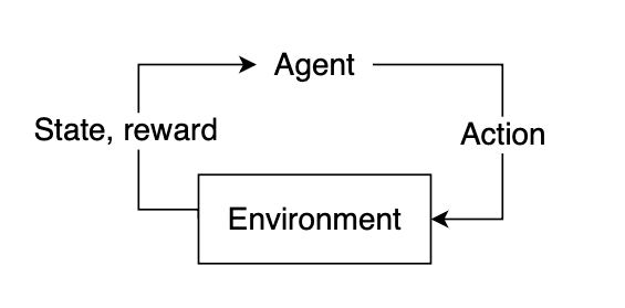
To pick a plan of action, our agent wants some details about the environment, given by the state. The state represents present details about the atmosphere, akin to place, velocity, time, and many others. Our agent doesn’t essentially know the whole lot of the present state. The data out there to our agent at any given cut-off date is known as an remark, which comprises some subset of knowledge current within the state. Not all states are absolutely observable, and a few states could require the agent to proceed realizing solely a small fraction of what may really be taking place within the atmosphere. Utilizing the remark, our agent should infer what the absolute best motion is perhaps primarily based on discovered expertise and try to pick out the motion that yields the best anticipated reward.
After deciding on an motion, the atmosphere will then reply by offering suggestions within the type of an up to date state and reward. This reward will assist us decide if the motion the agent took was optimum or not.
Markov Determination Processes (MDPs)
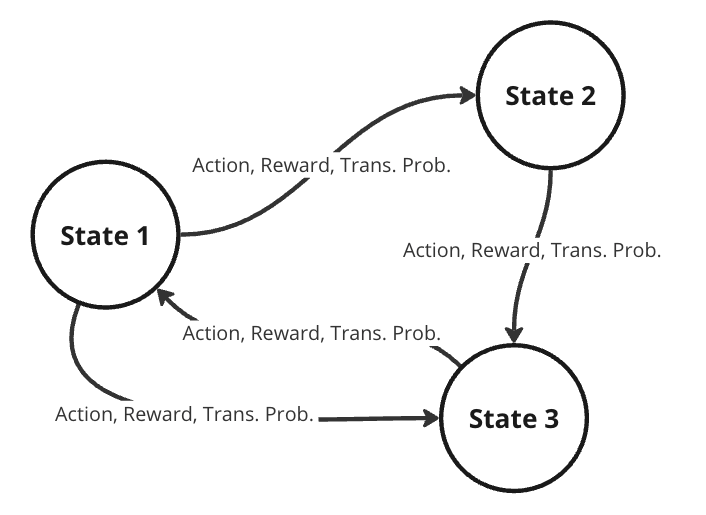
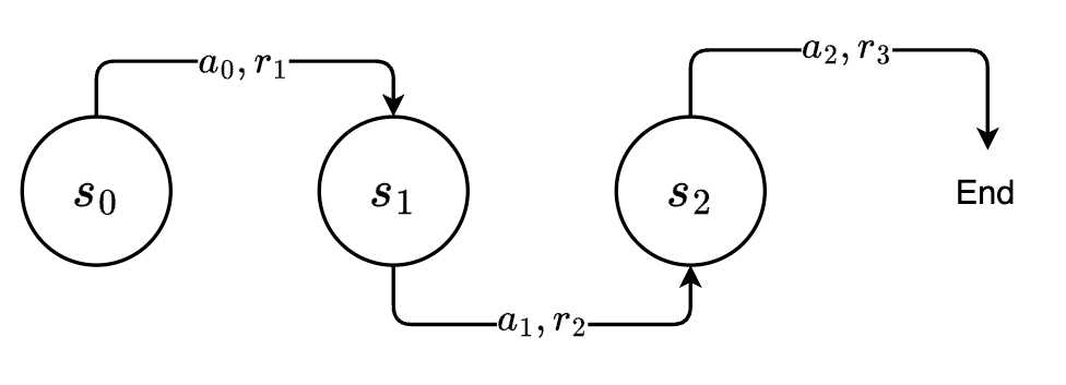
To raised characterize this drawback, we’d take into account it as a Markov determination course of (MDP). A MDP is a directed graph the place every edge within the graph has a non-deterministic property. At every doable state in our graph, now we have a set of actions we will select from, with every motion yielding some mounted reward and having some transitional chance of resulting in some subsequent state. Because of this the identical actions should not assured to result in the identical state each time for the reason that transition from one state to a different is just not solely depending on the motion, however the transitional chance as nicely.
Randomness in determination fashions is beneficial in sensible RL, permitting for dynamic environments the place the agent lacks full management. Flip-based video games like chess require the opponent to make a transfer earlier than you possibly can go once more. If the opponent performs randomly, the longer term state of the board is rarely assured, and our agent should play whereas accounting for a large number of various possible future states. When the agent takes some motion, the following state relies on what the opponent performs and is due to this fact outlined by a chance distribution throughout doable strikes for the opponent.
Our future state is due to this fact a perform of each the chance of the agent deciding on some motion and the transitional chance of the opponent deciding on some motion. On the whole, we will assume that for any atmosphere, the chance of our agent shifting to some subsequent state from our present state is denoted by the joint chance of the agent deciding on some motion and the transitional chance of shifting to that state.
Fixing the MDP
To find out the optimum plan of action, we wish to present our agent with a lot of expertise. By way of repeated iterations of the environment, we purpose to present the agent sufficient suggestions that it might probably accurately select the optimum motion most, if not all, of the time. Recall our definition of reinforcement studying: a studying course of constructed on the buildup of previous experiences coupled with quantifiable reward. After accumulating some expertise, we wish to use this expertise to higher choose our future actions.
We will quantify our experiences by utilizing them to foretell the anticipated reward from future states. As we accumulate extra expertise, our predictions will turn out to be extra correct, converging to the true worth after a sure variety of iterations. For every reward that we obtain, we will use that to replace some details about our state, so the following time we encounter this state, we’ll have a greater estimate of the reward that we’d count on to obtain.
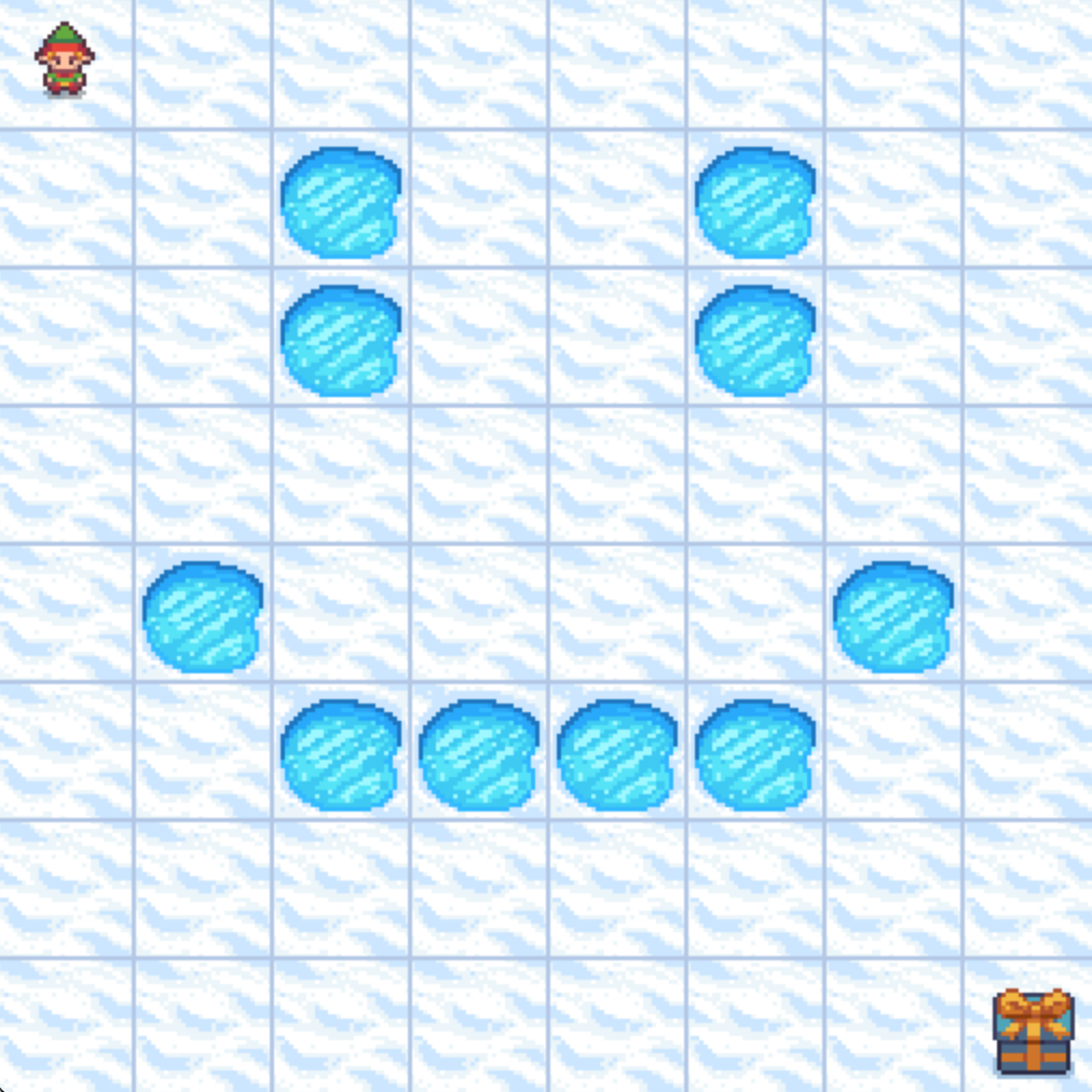
Frozen Lake Downside
Let’s take into account take into account a easy atmosphere the place our agent is a small character attempting to navigate throughout a frozen lake, represented as a 2D grid. It will probably transfer in 4 instructions: down, up, left, or proper. Our aim is to show it to maneuver from its begin place on the high left to an finish place positioned on the backside proper of the map whereas avoiding the holes within the ice. If our agent manages to efficiently attain its vacation spot, we’ll give it a reward of +1. For all different circumstances, the agent will obtain a reward of 0, with the added situation that if it falls right into a gap, the exploration will instantly terminate.

Every state might be denoted by its coordinate place within the grid, with the beginning place within the high left denoted because the origin (0, 0), and the underside proper ending place denoted as (3, 3).
Probably the most generic resolution could be to use some pathfinding algorithm to search out the shortest path to from high left to backside proper whereas avoiding holes within the ice. Nevertheless, the chance that the agent can transfer from one state to a different is just not deterministic. Every time the agent tries to maneuver, there’s a 66% likelihood that it’s going to “slip” and transfer to a random adjoining state. In different phrases, there’s solely a 33% likelihood of the motion the agent selected really occurring. A conventional pathfinding algorithm can’t deal with the introduction of a transitional chance. Due to this fact, we want an algorithm that may deal with stochastic environments, aka reinforcement studying.
This drawback can simply be represented as a MDP, with every state in our grid having some transitional chance of shifting to any adjoining state. To resolve our MDP, we have to discover the optimum plan of action from any given state. Recall that if we will discover a approach to precisely predict the longer term rewards from every state, we will greedily select the absolute best path by deciding on whichever state yields the highest anticipated reward. We’ll confer with this predicted reward because the state-value. Extra formally, the state-value will outline the anticipated reward gained ranging from some state plus an estimate of the anticipated rewards from all future states thereafter, assuming we act in line with the identical coverage of selecting the best anticipated reward. Initially, our agent may have no information of what rewards to count on, so this estimate might be arbitrarily set to 0.
Let’s now outline a approach for us to pick out actions for our agent to take: We’ll start with a desk to retailer our predicted state-value estimates for every state, containing all zeros.
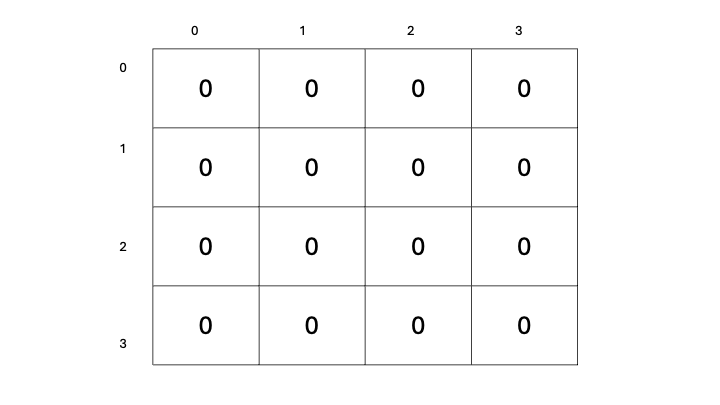
Our aim is to replace these state-value estimates as we discover the environment. The extra we traverse the environment, the extra expertise we may have, and the higher our estimates will turn out to be. As our estimates enhance, our state-values will turn out to be extra correct, and we may have a greater illustration of which states yield the next reward, due to this fact permitting us to pick out actions primarily based on which subsequent state has the best state-value. This may certainly work, proper?
State-value vs. Motion-value
Nope, sorry. One quick drawback that you simply may discover is that merely deciding on the following state primarily based on the best doable state-value isn’t going to work. After we take a look at the set of doable subsequent states, we aren’t contemplating our present motion—that’s, the motion that we are going to take from our present state to get to the following one. Primarily based on our definition of reinforcement studying, the agent-environment suggestions loop at all times consists of the agent taking some motion and the atmosphere responding with each state and reward. If we solely take a look at the state-values for doable subsequent states, we’re contemplating the reward that we might obtain ranging from these states, which fully ignores the motion (and consequent reward) we took to get there. Moreover, attempting to pick out a most throughout the following doable states assumes we will even make it there within the first place. Typically, being just a little extra conservative will assist us be extra constant in reaching the tip aim; nevertheless, that is out of the scope of this text :(.
As a substitute of evaluating throughout the set of doable subsequent states, we’d prefer to straight consider our out there actions. If our earlier state-value perform consisted of the anticipated rewards ranging from the following state, we’d prefer to replace this perform to now embody the reward from taking an motion from the present state to get to the following state, plus the anticipated rewards from there on. We’ll name this new estimate that features our present motion action-value.
We will now formally outline our state-value and action-value capabilities primarily based on rewards and transitional chance. We’ll use anticipated worth to characterize the connection between reward and transitional chance. We’ll denote our state-value as V and our action-value as Q, primarily based on customary conventions in RL literature.
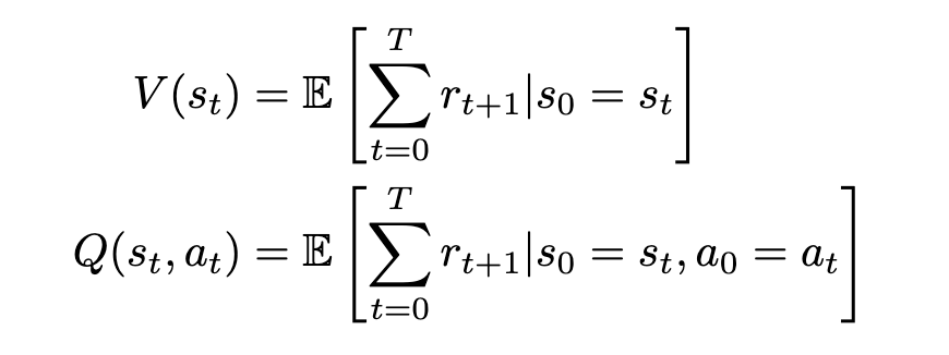
The state-value V of some state s[t] is the anticipated sum of rewards r[t] at every state ranging from s[t] to some future state s[T]; the action-value Q of some state s[t] is the anticipated sum of rewards r[t] at every state beginning by taking an motion a[t] to some future state-action pair s[T], a[T].
This definition is definitely not probably the most correct or typical, and we’ll enhance on it later. Nevertheless, it serves as a normal concept of what we’re in search of: a quantitative measure of future rewards.
Our state-value perform V is an estimate of the utmost sum of rewards r we might get hold of ranging from state s and regularly shifting to the states that give the best reward. Our action-value perform is an estimate of the utmost reward we might get hold of by taking motion from some beginning state and regularly selecting the optimum actions that yield the best reward thereafter. In each circumstances, we select the optimum motion/state to maneuver to primarily based on the anticipated reward that we might obtain and loop this course of till we both fall right into a gap or attain our aim.
Grasping Coverage & Return
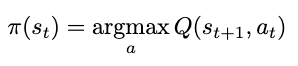
The strategy by which we select our actions is known as a coverage. The coverage is a perform of state—given some state, it’ll output an motion. On this case, since we wish to choose the following motion primarily based on maximizing the rewards, our coverage might be outlined as a perform returning the motion that yields the utmost action-value (Q-value) ranging from our present state, or an argmax. Since we’re at all times deciding on a most, we confer with this specific coverage as grasping. We’ll denote our coverage as a perform of state s: π(s), formally outlined as
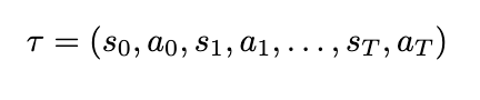
To simplify our notation, we will additionally outline a substitution for our sum of rewards, which we’ll name return, and a substitution for a sequence of states and actions, which we’ll name a trajectory. A trajectory, denoted by the Greek letter τ (tau), is denoted as
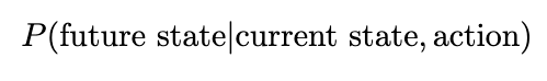
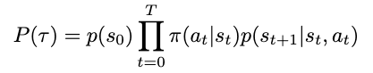
Since the environment is stochastic, it’s essential to additionally take into account the chance of such a trajectory occurring — low chance trajectories will cut back the expectation of reward. (Since our anticipated worth consists of multiplying our reward by the transitional chance, trajectories which are much less doubtless may have a decrease anticipated reward in comparison with excessive chance ones.) The chance might be derived by contemplating the chance of every motion and state taking place incrementally: At any timestep in our MDP, we’ll choose actions primarily based on our coverage, and the ensuing state might be depending on each the motion we chosen and the transitional chance. With out lack of generality, we’ll denote the transitional chance as a separate chance distribution, a perform of each the present state and the tried motion. The conditional chance of some future state occurring is due to this fact outlined as
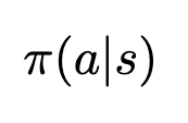
And the chance of some motion taking place primarily based on our coverage is just evaluated by passing our state into our coverage perform
Our coverage is at the moment deterministic, because it selects actions primarily based on the best anticipated action-value. In different phrases, actions which have a low action-value won’t ever be chosen, whereas actions with a excessive Q-value will at all times be chosen. This leads to a Bernoulli distribution throughout doable actions. That is very not often useful, as we’ll see later.
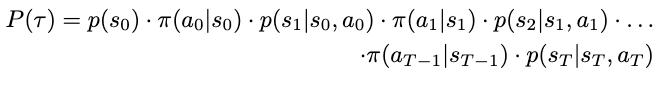
Making use of these expressions to our trajectory, we will outline the chance of some trajectory occurring as
For readability, right here’s the unique notation for a trajectory:
Extra concisely, we have
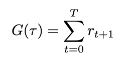
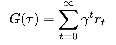
Defining each the trajectory and its chance permits us to substitute these expressions to simplify our definitions for each return and its anticipated worth. The return (sum of rewards), which we’ll outline as G primarily based on conventions, can now be written as
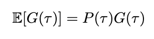
We will additionally outline the anticipated return by introducing chance into the equation. Since we’ve already outlined the chance of a trajectory, the anticipated return is due to this fact
We will now modify the definition of our price capabilities to incorporate the anticipated return
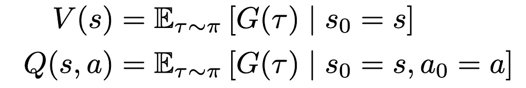
The primary distinction right here is the addition of the subscript τ∼π indicating that our trajectory was sampled by following our coverage (ie. our actions are chosen primarily based on the utmost Q-value). We’ve additionally eliminated the subscript t for readability. Right here’s the earlier equation once more for reference:
Discounted Return
So now now we have a reasonably well-defined expression for estimating return however earlier than we will begin iterating by means of the environment, there’s nonetheless some extra issues to think about. In our frozen lake, it’s pretty unlikely that our agent will proceed to discover indefinitely. In some unspecified time in the future, it’ll slip and fall right into a gap, and the episode will terminate. Nevertheless, in apply, RL environments may not have clearly outlined endpoints, and coaching classes may go on indefinitely. In these conditions, given an indefinite period of time, the anticipated return would strategy infinity, and evaluating the state- and action-value would turn out to be inconceivable. Even in our case, setting a tough restrict for computing return is oftentimes not useful, and if we set the restrict too excessive, we may find yourself with fairly absurdly giant numbers anyway. In these conditions, it is very important be sure that our reward sequence will converge utilizing a low cost issue. This improves stability within the coaching course of and ensures that our return will at all times be a finite worth no matter how far into the longer term we glance. Such a discounted return can be known as infinite horizon discounted return.
So as to add discounting to our return equation, we’ll introduce a brand new variable γ (gamma) to characterize the low cost issue.
Gamma should at all times be lower than 1, or our sequence is not going to converge. Increasing this expression makes this much more obvious
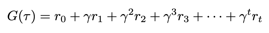
We will see that as time will increase, gamma might be raised to the next and better energy. As gamma is lower than 1, elevating it to the next exponent will solely make it smaller, thus exponentially lowering the contribution of future rewards to the general sum. We will substitute this up to date definition of return again into our price capabilities, although nothing will visibly change for the reason that variable remains to be the identical.
Exploration vs. Exploitation
We talked about earlier that at all times being grasping is just not your best option. All the time deciding on our actions primarily based on the utmost Q-value will in all probability give us the best likelihood of maximizing our reward, however that solely holds when now we have correct estimates of these Q-values within the first place. To acquire correct estimates, we want lots of info, and we will solely achieve info by attempting new issues — that’s, exploration.
After we choose actions primarily based on the best estimated Q-value, we exploit our present information base: we leverage our amassed experiences in an try to maximise our reward. After we choose actions primarily based on some other metric, and even randomly, we discover various potentialities in an try to realize extra helpful info to replace our Q-value estimates with. In reinforcement studying, we wish to stability each exploration and exploitation. To correctly exploit our information, we have to have information, and to realize information, we have to discover.
Epsilon-Grasping Coverage
We will stability exploration and exploitation by altering our coverage from purely grasping to an epsilon-greedy one. An epsilon-greedy coverage acts greedily more often than not with a chance of 1- ε, however has a chance of ε to behave randomly. In different phrases, we’ll exploit our information more often than not in an try to maximise reward, and we’ll discover often to realize extra information. This isn’t the one approach of balancing exploration and exploitation, but it surely is without doubt one of the easiest and best to implement.
Abstract
Now the we’ve established a foundation for understanding RL rules, we will transfer to discussing the precise algorithm — which can occur within the subsequent article. For now, we’ll go over the high-level overview, combining all these ideas right into a cohesive pseudo-code which we will delve into subsequent time.
Q-Studying
The main target of this text was to ascertain the idea for understanding and implementing Q-learning. Q-learning consists of the next steps:
- Initialize a tabular estimate of all action-values (Q-values), which we replace as we iterate by means of the environment.
- Choose an motion by sampling from our epsilon-greedy coverage.
- Acquire the reward (if any) and replace our estimate for our action-value.
- Transfer to the following state, or terminate if we fall right into a gap or attain the aim.
- Loop steps 2–4 till our estimated Q-values converge.
Q-learning is an iterative course of the place we construct estimates of action-value (and anticipated return), or “expertise”, and use our experiences to determine which actions are probably the most rewarding for us to decide on. These experiences are “discovered” over many successive iterations of the environment and by leveraging them we can constantly attain our aim, thus fixing our MDP.
Glossary
- Atmosphere — something that can not be arbitrarily modified by our agent, aka the world round it
- State — a selected situation of the atmosphere
- Remark — some subset of knowledge from the state
- Coverage — a perform that selects an motion given a state
- Agent — our “learner” which acts in line with a coverage in the environment
- Reward — what our agent receives after performing sure actions
- Return — a sum of rewards throughout a sequence of actions
- Discounting — the method by means of which we be sure that our return doesn’t attain infinity
- State-value — the anticipated return ranging from a state and persevering with to behave in line with some coverage, perpetually
- Motion-value — the anticipated return ranging from a state and taking some motion, after which persevering with to behave in line with some coverage, perpetually
- Trajectory — a sequence of states and actions
- Markov Determination Course of (MDP) — the mannequin we use to characterize determination issues in RL aka a directed graph with non-deterministic edges
- Exploration — how we get hold of extra information
- Exploitation — how we use our present information base to realize extra reward
- Q-Studying — a RL algorithm the place we iteratively replace Q-values to acquire higher estimates of which actions will yield increased anticipated return
- Reinforcement Studying — a studying course of constructed on the buildup of previous experiences coupled with quantifiable reward
In the event you’ve learn this far, take into account leaving some suggestions concerning the article — I’d admire it ❤.
References
[1] Gymnasium, Frozen Lake (n.d.), OpenAI Gymnasium Documentation.
[2] OpenAI, Spinning Up in Deep RL (n.d.), OpenAI.
[3] R. Sutton and A. Barto, Reinforcement Studying: An Introduction (2020), http://incompleteideas.web/guide/RLbook2020.pdf
[4] Spiceworks, What’s a Markov Determination Course of? (n.d.), Spiceworks
[5] IBM, Reinforcement Studying (n.d.), IBM
An Intuitive Introduction to Reinforcement Studying, Half I was initially printed in In the direction of Information Science on Medium, the place individuals are persevering with the dialog by highlighting and responding to this story.


