


Enhance accuracy, pace, and reminiscence utilization by performing PCA transformation earlier than outlier detection
21 hours in the past
This text continues a sequence associated to functions of PCA (precept part evaluation) for outlier detection, following Utilizing PCA for Outlier Detection. That article described PCA itself, and launched the 2 fundamental methods we are able to use PCA for outlier detection: evaluating the reconstruction error, and operating commonplace outlier detectors on the PCA-transformed area. It additionally gave an instance of the primary strategy, utilizing reconstruction error, which is easy to do utilizing the PCA and KPCA detectors offered by PyOD.
This text covers the second strategy, the place we first remodel the information area utilizing PCA after which run commonplace outlier detection on this. As lined within the earlier article, this could in some circumstances decrease interpretability, but it surely does have some shocking advantages when it comes to accuracy, execution time, and reminiscence utilization.
This text can be half of a bigger sequence on outlier detection, to date protecting FPOF, Counts Outlier Detector, Distance Metric Studying, Shared Nearest Neighbors, and Doping. This text additionally contains one other excerpt from my guide Outlier Detection in Python.
In the event you’re moderately conversant in PCA itself (because it’s used for dimensionality discount or visualization), you possibly can most likely skip the earlier article if you want, and dive straight into this one. I’ll, although, in a short time evaluate the principle thought.
PCA is a way to remodel information (viewing information data as factors in high-dimensional area) from one set of coordinates to a different. If we begin with a dataset (as proven under within the left pane), with 100 data and two options, then we are able to view the information as 100 factors in 2-dimensional area. With extra life like information, we might have many extra data and plenty of extra dimensions, however the identical thought holds. Utilizing PCA, we transfer the information to a brand new set of coordinates, so successfully create a brand new set of options describing every report. As described within the earlier article, that is accomplished by figuring out orthogonal traces by way of the information (proven within the left pane because the blue and orange traces) that match the information properly.
So, if we begin with a dataset, reminiscent of is proven within the left pane under, we are able to apply PCA transformation to remodel the information into one thing like is proven in the precise pane. In the precise pane, we present the 2 PCA elements the information was mapped to. The elements are merely named 0 and 1.

One factor to notice about PCA elements is that they’re utterly uncorrelated. This can be a results of how they’re constructed; they’re primarily based on traces, planes, or hyperplanes by way of the unique information which are all strictly orthogonal to one another. We will see in the precise pane, there isn’t a relationship between part 0 and part 1.
This has robust implications for outlier detection; specifically it implies that outliers are typically remodeled into excessive values in a number of of the elements, and so are simpler to detect. It additionally implies that extra subtle outlier checks (that check for uncommon associations among the many options) are usually not vital, and less complicated checks can be utilized.
Earlier than trying nearer at the advantages of PCA for for outlier detection, I’ll shortly go over two forms of outlier detectors. There are a lot of methods to categorise outlier detection algorithms, however one helpful approach is to differentiate between what are known as univariate from multivariate checks.
Univariate Assessments
The time period univariate refers to checks that simply examine one characteristic — checks that determine the uncommon or excessive values in that one characteristic. Examples are checks primarily based on z-score, interquartile vary (IQR), inter-decile vary (IDR), median absolute deviation (MAD), histogram checks, KDE checks, and so forth.
One histogram-based check offered by PyOD (PyOD might be probably the most full and great tool for outlier detection on tabular information accessible in Python immediately) is HBOS (Histogram-based Outlier Rating — described in my Medium article on Counts Outlier Detector, and intimately in Outlier Detection in Python).
As lined in Utilizing PCA for Outlier Detection, one other univariate check offered by PyOD is ECOD.
To explain univariate checks, we take a look at an instance of outlier detection for a particular real-world dataset. The next desk is a subset of the baseball dataset from OpenML (accessible with a public license), right here exhibiting simply three rows and 5 columns (there are a number of extra options within the full dataset). Every row represents one participant, with statistics for every, together with the variety of seasons they performed, variety of video games, and so forth.

To determine uncommon gamers, we are able to search for these data with uncommon single values (for instance, gamers that performed in unusually many seasons, had unusually many At bats, and so forth). These can be discovered with univariate checks.
For instance, utilizing z-score checks to search out uncommon data, we might truly carry out a z-score check on every column, one by one. We’d first examine the Quantity seasons column (assessing how uncommon every worth within the column is relative to that column), then the Video games performed column and so forth.
When checking, for instance, the Quantity seasons column, utilizing a z-score check, we might first decide the imply and commonplace deviation of the column. (Different checks could decide the median and interquartile vary for the column, histogram bin counts, and so forth.).
We might then decide absolutely the z-score for every worth within the Quantity seasons column: the variety of commonplace deviations every worth is from the imply. The bigger the z-score, the extra uncommon the worth. Any values with an absolute z-score over about 4.0 or 5.0 can seemingly be thought-about anomalous, although this relies on the dimensions of the information and the distribution.
We’d then repeat this for one another column. As soon as that is accomplished, we’ve got, for every row, a rating for a way uncommon every worth within the row is relative to their columns. So, every row would have a set of scores: one rating for every worth in that row.
We then want to find out an total outlier rating for every report. There are other ways to do that, and a few nuances related to every, however two easy strategies are to take the typical z-score of the values per row, or to take the utmost z-score per row.
Multivariate Assessments
Multivariate checks contemplate a number of options without delay. In actual fact, virtually all multivariate outlier detectors contemplate all options without delay.
Nearly all of outlier detectors (together with Isolation Forest, Native Outlier Issue (LOF), KNN, and so forth) are primarily based on multivariate checks.
The benefit of those detectors is, we are able to search for data with uncommon combos of values. For instance, some gamers could have a typical variety of Runs and a typical variety of At bats, however could have unusually many (or presumably unusually few) Runs given their variety of At bats. These can be discovered with multivariate checks.
Within the scatter plot above (contemplating the unique information within the left pane), Level A is excessive in each dimensions, so could possibly be detected by a univariate check. In actual fact, a univariate check on Characteristic A would seemingly flag Level A, and a univariate check on Characteristic B would seemingly as properly, and so Level A, being anomalous in each options, can be scored extremely utilizing univariate checks.
Level B, although, is typical in each dimensions. Solely the mix of values is uncommon, and to detect this as an anomaly, we might require a multivariate check.
Usually, when performing outlier detection on tabular information, we’re searching for uncommon rows, versus uncommon single values. And, uncommon rows will embrace each these rows with uncommon single values, in addition to uncommon combos of values. So, each univariate and multivariate checks are sometimes helpful. Nevertheless, multivariate checks will catch each univariate and multivariate outliers (within the scatter plot, a multivariate check reminiscent of Isolation Forest, LOF, or KNN would usually catch each Level A and Level B), and so in follow, multivariate checks are typically used extra typically.
However, in outlier detection will we very often restrict evaluation to univariate checks. Univariate checks are sooner — typically a lot sooner (which may be crucial in real-time environments, or environments the place there are very massive volumes of information to evaluate). Univariate checks additionally are typically extra interpretable.
They usually don’t undergo from the curse of dimensionality. That is lined in Counts Outlier Detector, Shared Nearest Neighbors, and Outlier Detection in Python, however the normal thought is that multivariate checks can break down when working with too many options. That is for a lot of causes, however an necessary one is that distance calculations (which many outlier detectors, together with LOF and KNN, depend on) can develop into meaningless given sufficient dimensions. Typically working with simply 20 or extra options, and fairly often with about 50 or extra, outlier scores can develop into unreliable.
Univariate checks scale to larger dimensions significantly better than multivariate checks, as they don’t depend on distance calculations between the rows.
And so, there are some main benefits to utilizing univariate checks. However, additionally some main disadvantages: these miss outliers that relate to uncommon combos of values, and so can detect solely a portion of the related outliers.
So, in most contexts, it’s helpful (and extra frequent) to run multivariate checks. However, they’re slower, much less interpretable, and extra inclined to the curse of dimensionality.
An attention-grabbing impact of PCA transformation is that univariate checks develop into rather more sensible. As soon as PCA transformation is finished, there are not any associations between the options, and so there isn’t a idea of surprising combos of values.
Within the scatter plot above (proper pane — after the PCA transformation), we are able to see that Factors A and B can each be recognized merely as excessive values. Level A is excessive in Part 0; Level B is excessive in Part 1.
Which suggests, we are able to carry out outlier detection successfully utilizing easy statistical checks, reminiscent of z-score, IQR, IDR or MAD checks, or utilizing easy instruments reminiscent of HBOS and ECOD.
Having stated that, it’s additionally attainable, after reworking the dataspace utilizing PCA, to nonetheless use commonplace multivariate checks reminiscent of Isolation Forest, LOF, or another commonplace instruments. If these are the instruments we mostly use, there’s a comfort to persevering with to make use of them, and to easily first remodel the information utilizing PCA as a pre-processing step.
One benefit they supply over statistical strategies (reminiscent of z-score, and so forth.) is that they mechanically present a single outlier rating for every report. If we use z-score checks on every report, and the information has, say, 20 options and we convert this to 10 elements (it’s attainable to not use all elements, as described under), then every report could have 10 outlier scores — one associated to how uncommon it’s in every of the ten elements used. It’s then vital to mix these scores right into a single outlier rating. As indicated above, there are easy methods to do that (together with taking the imply, median, or most z-score for every worth per row), however there are some problems doing this (as lined in Outlier Detection in Python). That is fairly manageable, however having a detector present a single rating is handy as properly.
We’ll now take a look at an instance utilizing PCA to assist higher determine outliers in a dataset. To make it simpler to see how outlier detection works with PCA, for this instance we’ll create two fairly simple artificial datasets. We’ll create each with 100,000 rows and 10 options. And we add some identified outliers, considerably just like Factors A and B within the scatter plot above.
We restrict the datasets to 10 options for simplicity, however as urged above and within the earlier article, there may be robust advantages to utilizing PCA in high-dimensional area, and so (although it’s not lined on this instance), extra of a bonus to utilizing PCA with, say, a whole lot of options, than ten. The datasets used right here, although, are moderately simple to work with and to know.
The primary dataset, data_corr, is created to have robust associations (correlations) between the options. We replace the final row to include some massive (however not exceptionally massive) values. The principle factor is that this row deviates from the conventional patterns between the options.
We create one other check dataset known as data_extreme, which has no associations between the options. The final row of that is modified to include excessive values in some options.
This permits us to check with two well-understood information distributions in addition to well-understood outlier varieties (we’ve got one outlier in data_corr that ignores the conventional correlations between the options; and we’ve got one outlier in data_extreme that has excessive values in some options).
This instance makes use of a number of PyOD detectors, which requires first executing:
pip set up pyod
The code then begins with creating the primary check dataset:
import numpy as np
import pandas as pd
from sklearn.decomposition import PCA
from pyod.fashions.ecod import ECOD
from pyod.fashions.iforest import IForest
from pyod.fashions.lof import LOF
from pyod.fashions.hbos import HBOS
from pyod.fashions.gmm import GMM
from pyod.fashions.abod import ABOD
import timenp.random.seed(0)
num_rows = 100_000
num_cols = 10
data_corr = pd.DataFrame({0: np.random.random(num_rows)})
for i in vary(1, num_cols):
data_corr[i] = data_corr[i-1] + (np.random.random(num_rows) / 10.0)
copy_row = data_corr[0].argmax()
data_corr.loc[num_rows-1, 2] = data_corr.loc[copy_row, 2]
data_corr.loc[num_rows-1, 4] = data_corr.loc[copy_row, 4]
data_corr.loc[num_rows-1, 6] = data_corr.loc[copy_row, 6]
data_corr.loc[num_rows-1, 8] = data_corr.loc[copy_row, 8]
start_time = time.process_time()
pca = PCA(n_components=num_cols)
pca.match(data_corr)
data_corr_pca = pd.DataFrame(pca.remodel(data_corr),
columns=[x for x in range(num_cols)])
print("Time for PCA tranformation:", (time.process_time() - start_time))
We now have the primary check dataset, data_corr. When creating this, we set every characteristic to be the sum of the earlier options plus some randomness, so all options are well-correlated. The final row is intentionally set as an outlier. The values are massive, although not exterior of the present information. The values within the identified outlier, although, don’t comply with the conventional patterns between the options.
We then calculate the PCA transformation of this.
We subsequent do that for the opposite check dataset:
np.random.seed(0)data_extreme = pd.DataFrame()
for i in vary(num_cols):
data_extreme[i] = np.random.random(num_rows)
copy_row = data_extreme[0].argmax()
data_extreme.loc[num_rows-1, 2] = data_extreme[2].max() * 1.5
data_extreme.loc[num_rows-1, 4] = data_extreme[4].max() * 1.5
data_extreme.loc[num_rows-1, 6] = data_extreme[6].max() * 1.5
data_extreme.loc[num_rows-1, 8] = data_extreme[8].max() * 1.5
start_time = time.process_time()
pca = PCA(n_components=num_cols)
pca.match(data_corr)
data_extreme_pca = pd.DataFrame(pca.remodel(data_corr),
columns=[x for x in range(num_cols)])
print("Time for PCA tranformation:", (time.process_time() - start_time))
Right here every characteristic is created independently, so there are not any associations between the options. Every characteristic merely follows a uniform distribution. The final row is ready as an outlier, having excessive values in options 2, 4, 6, and eight, so in 4 of the ten options.
We now have each check datasets. We subsequent outline a operate that, given a dataset and a detector, will prepare the detector on the total dataset in addition to predict on the identical information (so will determine the outliers in a single dataset), timing each operations. For the ECOD (empirical cumulative distribution) detector, we add particular dealing with to create a brand new occasion in order to not keep a reminiscence from earlier executions (this isn’t vital with the opposite detectors):
def evaluate_detector(df, clf, model_type):
"""
params:
df: information to be assessed, in a pandas dataframe
clf: outlier detector
model_type: string indicating the kind of the outlier detector
"""international scores_df
if "ECOD" in model_type:
clf = ECOD()
start_time = time.process_time()
clf.match(df)
time_for_fit = (time.process_time() - start_time)
start_time = time.process_time()
pred = clf.decision_function(df)
time_for_predict = (time.process_time() - start_time)
scores_df[f'{model_type} Scores'] = pred
scores_df[f'{model_type} Rank'] =
scores_df[f'{model_type} Scores'].rank(ascending=False)
print(f"{model_type:<20} Match Time: {time_for_fit:.2f}")
print(f"{model_type:<20} Predict Time: {time_for_predict:.2f}")
The following operate outlined executes for every dataset, calling the earlier technique for every. Right here we check 4 circumstances: utilizing the unique information, utilizing the PCA-transformed information, utilizing the primary 3 elements of the PCA-transformed information, and utilizing the final 3 elements. This may inform us how these 4 circumstances evaluate when it comes to time and accuracy.
def evaluate_dataset_variations(df, df_pca, clf, model_name):
evaluate_detector(df, clf, model_name)
evaluate_detector(df_pca, clf, f'{model_name} (PCA)')
evaluate_detector(df_pca[[0, 1, 2]], clf, f'{model_name} (PCA - 1st 3)')
evaluate_detector(df_pca[[7, 8, 9]], clf, f'{model_name} (PCA - final 3)')
As described under, utilizing simply the final three elements works properly right here when it comes to accuracy, however in different circumstances, utilizing the early elements (or the center elements) can work properly. That is included right here for instance, however the the rest of the article will focus simply on the choice of utilizing the final three elements.
The ultimate operate outlined known as for every dataset. It executes the earlier operate for every detector examined right here. For this instance, we use six detectors, every from PyOD (Isolation Forest, LOF, ECOD, HBOS, Gaussian Combination Fashions (GMM), and Angle-based Outlier Detector (ABOD)):
def evaluate_dataset(df, df_pca):
clf = IForest()
evaluate_dataset_variations(df, df_pca, clf, 'IF')clf = LOF(novelty=True)
evaluate_dataset_variations(df, df_pca, clf, 'LOF')
clf = ECOD()
evaluate_dataset_variations(df, df_pca, clf, 'ECOD')
clf = HBOS()
evaluate_dataset_variations(df, df_pca, clf, 'HBOS')
clf = GMM()
evaluate_dataset_variations(df, df_pca, clf, 'GMM')
clf = ABOD()
evaluate_dataset_variations(df, df_pca, clf, 'ABOD')
We lastly name the evaluate_dataset() technique for each check datasets and print out the highest outliers (the identified outliers are identified to be within the final rows of the 2 check datasets):
# Take a look at the primary dataset
# scores_df shops the outlier scores given to every report by every detector
scores_df = data_corr.copy()
evaluate_dataset(data_corr, data_corr_pca)
rank_columns = [x for x in scores_df.columns if type(x) == str and 'Rank' in x]
print(scores_df[rank_columns].tail())# Take a look at the second dataset
scores_df = data_extreme.copy()
evaluate_dataset(data_extreme, data_extreme_pca)
rank_columns = [x for x in scores_df.columns if type(x) == str and 'Rank' in x]
print(scores_df[rank_columns].tail())
There are a number of attention-grabbing outcomes. We glance first on the match occasions for the data_corr dataset, proven in desk under (the match and predict occasions for the opposite check set had been comparable, so not proven right here). The checks had been carried out on Google colab, with the occasions proven in seconds. We see that completely different detectors have fairly completely different occasions. ABOD is considerably slower than the others, and HBOS significantly sooner. The opposite univariate detector included right here, ECOD, can be very quick.
The occasions to suit the PCA-transformed information are about the identical as the unique information, which is sensible given this information is identical dimension: we transformed the ten options to 10 elements, that are equal, when it comes to time, to course of.
We additionally check utilizing solely the final three PCA elements (elements 7, 8, and 9), and the match occasions are drastically diminished in some circumstances, significantly for native outlier issue (LOF). In comparison with utilizing all 10 authentic options (19.4s), or utilizing all 10 PCA elements (16.9s), utilizing 3 elements required just one.4s. In all circumstances as well0, aside from Isolation Forest, there’s a notable drop in match time.

Within the subsequent desk, we see the predict occasions for the data_corr dataset (the occasions for the opposite check set had been comparable right here as properly). Once more, we see a really sizable drop in prediction occasions utilizing simply three elements, particularly for LOF. We additionally see once more that the 2 univariate detectors, HBOS and ECOD had been among the many quickest, although GMM is as quick or sooner within the case of prediction (although barely slower when it comes to match time).
With Isolation Forest (IF), as we prepare the identical variety of timber whatever the variety of options, and go all data to be evaluated by way of the identical set of timber, the occasions are unaffected by the variety of options. For all different detectors proven right here, nevertheless, the variety of options may be very related: all others present a big drop in predict time when utilizing 3 elements in comparison with all 10 authentic options or all 10 elements.

When it comes to accuracy, all 5 detectors carried out properly on the 2 datasets more often than not, when it comes to assigning the very best outlier rating to the final row, which, for each check datasets, is the one identified outlier. The outcomes are proven within the subsequent desk. There are two rows, one for every dataset. For every, we present the rank assigned by every detector to the one identified outlier. Ideally, all detectors would assign this rank 1 (the very best outlier rating).
Generally, the final row was, in truth, given the very best or practically highest rank, excluding IF, ECOD, and HBOS on the primary dataset. This can be a good instance the place even robust detectors reminiscent of IF can often do poorly even for clear outliers.

For the primary dataset, ECOD and HBOS utterly miss the outlier, however that is as anticipated, as it’s an outlier primarily based on a mix of values (it ignores the conventional linear relationship among the many options), which univariate checks are unable to detect. The second dataset’s outlier is predicated on excessive values, which each univariate and multivariate checks are sometimes in a position to detect reliably, and might accomplish that right here.
We see a drastic enchancment in accuracy when utilizing PCA for these datasets and these detectors, proven within the subsequent desk. This isn’t at all times the case, but it surely does maintain true right here. When the detectors execute on the PCA-transformed information, all 6 detectors rank the identified outlier the very best on each datasets. When information is PCA-transformed, the elements are all unassociated with one another; the outliers are the acute values, that are a lot simpler to determine.

Additionally attention-grabbing is that solely the final three elements are essential to rank the identified outliers as the highest outliers, proven within the desk right here.
And, as we noticed above, match and predict occasions are considerably shorter in these circumstances. That is the place we are able to obtain vital efficiency enhancements utilizing PCA: it’s typically vital to make use of solely a small variety of the elements.
Utilizing solely a small set of elements may also cut back reminiscence necessities. This isn’t at all times a problem, however typically when working with massive datasets, this may be an necessary consideration.
This experiment lined two of the principle forms of outliers we are able to have with information: excessive values and values that deviate from a linear sample, each of that are identifiable within the later elements. In these circumstances, utilizing the final three elements labored properly.
It could possibly differ what number of elements to make use of, and which elements are finest to make use of, and a few experimentation can be wanted (seemingly finest found utilizing doped information). In some circumstances, it could be preferable (when it comes to execution time, detecting the related outliers reliably, and lowering noise) to make use of the sooner elements, in some circumstances the center, and in some circumstances the later. As we are able to see within the scatter plot in the beginning of this text, completely different elements can have a tendency to spotlight several types of outlier.
One other helpful advantage of working with PCA elements is that it may well make it simpler to tune the outlier detection system over time. Typically with outlier detection, the system is run not simply as soon as on a single dataset, however on an ongoing foundation, so continuously assessing new information because it arrives (for instance, new monetary transactions, sensor readings, website online logs, community logs, and so forth.), and over time we achieve a greater sense of what outliers are most related to us, and that are being under- and over-reported.
Because the outliers reported when working with PCA-transformed information all relate to a single part, we are able to see what number of related and irrelevant outliers being reported are related to every part. This may be significantly simple when utilizing easy univariate checks on every part, like z-score, IQR, IDR, MAD-based checks, and comparable checks.
Over time, we are able to study to weight outliers related to some elements extra extremely and different elements decrease (relying on our tolerance for false constructive and false negatives).
Dimensionality discount additionally has some benefits in that it may well assist visualize the outliers, significantly the place we cut back the information to 2 or three dimensions. Although, as with the unique options, even the place there are greater than three dimensions, we are able to view the PCA elements one by one within the type of histograms, or two at a time in scatter plots.
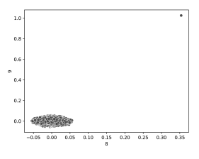
For instance, inspecting the final two elements of the primary check dataset, data_corr (which contained uncommon combos of values) we are able to see the identified outlier clearly, as proven under. Nevertheless, it’s considerably questionable how informative that is, because the elements themselves are obscure.

This text lined PCA, however there are different dimensionality discount instruments that may be equally used, together with t-SNE (as with PCA, that is offered in scikit-learn), UMAP, and auto-encoders (additionally lined in Outlier Detection in Python).
As properly, utilizing PCA, strategies primarily based on reconstruction error (measuring how properly the values of a report may be approximated utilizing solely a subset of the elements) may be very efficient and is usually price investigating, as lined within the earlier article on this sequence.
This text lined utilizing commonplace outlier detectors (although, as demonstrated, this could extra readily embrace easy univariate outlier detectors than is often attainable) for outlier detection, exhibiting the advantages of first reworking the information utilizing PCA.
How properly this course of will work relies on the information (for instance, PCA depends on there being robust linear relationships between the options, and might breakdown if the information is closely clustered) and the forms of outliers you’re all in favour of discovering. It’s normally vital to make use of doping or different types of testing to find out how properly this works, and to tune the method — significantly figuring out which elements are used. The place there are not any constraints associated to execution time or reminiscence limits although, it may be a great place to begin to easily use all elements and weight them equally.
As properly, in outlier detection, normally no single outlier detection course of will reliably determine all of the forms of outliers you’re all in favour of (particularly the place you’re all in favour of discovering all data that may be moderately thought-about statistically uncommon in a method or one other), and so a number of outlier detection strategies usually must be used. Combining PCA-based outlier detection with different strategies can cowl a wider vary of outliers than may be detected utilizing simply PCA-based strategies, or simply strategies with out PCA transformations.
However, the place PCA-based strategies work properly, they’ll typically present extra correct detection, because the outliers are sometimes higher separated and simpler to detect.
PCA-based strategies can even execute extra shortly (significantly the place they’re enough and don’t must be mixed with different strategies), as a result of: 1) less complicated (and sooner) detectors reminiscent of z-score, IQR, HBOS and ECOD can be utilized; and a pair of) fewer elements could also be used. The PCA transformations themselves are usually extraordinarily quick, with occasions virtually negligible in comparison with becoming or executing outlier detection.
Utilizing PCA, at the least the place solely a subset of the elements are vital, can even cut back reminiscence necessities, which may be a problem when working with significantly massive datasets.
All pictures by writer


