Mannequin Predictive Management Fundamentals | In direction of Information Science

Why AI Nonetheless Can’t Substitute Analysts: A Predictive Upkeep Instance

TDS E-newsletter: September Should-Reads on ML Profession Roadmaps, Python Necessities, AI Brokers, and Extra

Fast

On this article we’ll:

1. Introduction

Mannequin predictive management (MPC) is a well-liked suggestions management methodology the place a finite-horizon optimum management drawback (OCP) is iteratively solved with an up to date measured state on every iteration.

Within the OCP one makes use of a mannequin of the plant to search out the optimum open loop management over the finite horizon thought-about. As a result of the mannequin can’t seize the true plant’s behaviour 100%, and since in the true world the system is subjected to noise and disturbances, one solely applies the primary portion of the optimum open loop management, and recurrently measures the state to re-solve the OCP. This closes the loop and creates a suggestions.

The maths behind it’s comparatively easy and intuitive (particularly when in comparison with issues like strong management) and it’s simple to code up an MPC controller. Different execs are that it could actually successfully deal with onerous and tender constraints on the state and management (onerous constraints are strict, whereas tender constraints are enforced by way of penalisation in the associated fee operate) and it could actually typically be used on nonlinear techniques with nonconvex constraints (relying on how nasty these are after all!). The one con is that you must resolve a optimization issues “on-line” in actual time, which could be a drawback for those who’re controlling a quick system or have restricted computing assets.

1.2 Working Instance

All through the article I’ll contemplate the double integrator with a zero-order maintain management (i.e. a piecewise fixed management) because the operating instance within the code. The continual time system reads:

[
begin{align*}
dot x _1(t) & = x_2(t),
dot x _2(t) & = u(t),
end{align*}
]

with (t in mathbb{R} ) denoting time. Right here ( x_1(t) in mathbb{R} ) is the place whereas ( x_2(t) in mathbb{R} ) is the velocity. You may consider this technique as a 1kg block sliding on a frictionless desk, with (u(t)) the utilized drive.

Working instance: the double integrator. Picture by writer.

If we constrain the management to be piecewise fixed over intervals of size 0.1 seconds, we get the discrete-time system:

[
begin{align*}
x_{k+1} &= A x_k + Bu_k,
end{align*}
]

with (ok in mathbb{Z}), the place,

[
begin{align*}
A :=
left(
begin{array}{cc}
1 & 0.1
0 & 1
end{array}
right), ,,
B :=
left(
begin{array}{c}
0.05
1
end{array}
right)
end{align*}
]

and (x_k in mathbb{R}^2 ), (u_k in mathbb{R} ). (Observe that I take advantage of (x_k) and (u_k) to discuss with the discrete-time system’s state and management to make the notation neater in the remainder of the article.)

You should utilize the scipy packages’s cont2discrete operate to get this discrete time system, as follows:

import numpy as np
from scipy.sign import cont2discrete

A = np.array([[0, 1],[0, 0]])
B = np.array([[0],[1]])
C = np.array([[1, 0],[0, 1]])
D = np.array([[0, 0],[0, 0]])
dt = 0.1 # in seconds
discrete_system = cont2discrete((A, B, C, D), dt, methodology='zoh')
A_discrete, B_discrete, *_ = discrete_system

2. Optimum Management Drawback

We’ll contemplate the next discrete-time optimum management drawback (OCP):

[
begin{equation}
{mathrm{OCP}(bar x):}begin{cases}
minlimits_{mathbf{u},mathbf{x}} quad & sum_{k=0}^{K-1} left(x_k^{top}Qx_k + u_k^top R u_k right)+ x_{K}^top Q_K x_{K}
mathrm{subject to:}quad & x_{k+1} = Ax_k + Bu_k, &k in[0:K-1], & dots(1)
quad & x_0 = bar x , & & dots(2)
quad & x_kin [-1,1]instances(-infty,infty),& ok in[1:K], & dots(3)
quad & u_kin [-1,1],& ok in[0:K-1], & dots(4)
finish{circumstances}
finish{equation}
]

the place,

(Kinmathbb{R}_{geq 0}) denotes the finite horizon over which we resolve the OCP,
(kinmathbb{Z}) denotes the discrete time step,
([p:q]), with (p,qinmathbb{Z}), denotes the set of integers ({p,p+1,…,q}),
(bar x in mathbb{R}^2 ) denotes the preliminary situation of the dynamical system,
(x_kinmathbb{R}^2 ) denotes the state at step (ok),
(uinmathbb{R}) denotes the management at step (ok),
(Qinmathbb{R}^{2times 2}), (Rinmathbb{R}) and (Q_K in mathbb{R}^{2times 2}) are sq. constructive particular matrices that specify the associated fee operate ((R) is scalar right here as a result of (u) is scalar).

Furthermore, we’ll let,

(mathbf{u}:= (u_0,u_1,…,u_{Ok−1})inmathbb{R}^Ok ) denote the management sequence,
(mathbf{x}:= (x_0,x_1,…,x_{Ok})inmathbb{R}^{2(Ok+1)} ) denote the state sequence.

To be rigorous, we’ll say that the pair ((mathbf{u}^{*}, mathbf{x}^{*})inmathbb{R}^Ok instances mathbb{R}^{2(Ok+1)}) is a resolution to ( mathrm{OCP}(bar{x})) supplied that it minimises the associated fee operate over all admissible pairs, that’s,

[
begin{equation*}
J(mathbf{u}^{*}, mathbf{x}^{*}) leq J(mathbf{u}, mathbf{x}),quad forall (mathbf{u},mathbf{x})in Omega
end{equation*}
]

the place (J:mathbb{R}^Ok instances mathbb{R}^{2(Ok+1)}rightarrow mathbb{R}_{geq 0} ) is,

[
begin{equation*}
J(mathbf{u},mathbf{x}) :=left( sum_{k=0}^{K-1 }x_k^top Q x_k + u_k^top R u_k right) + x_K^top Q_K x_K
end{equation*}
]

and (Omega ) denotes all admissible pairs,

[
Omega :={(mathbf{u},mathbf{x})in mathbb{R}^{K}times mathbb{R}^{2(K+1)} : (1)-(4),, mathrm{hold}}.
]

Thus, the optimum management drawback is to discover a management and state sequence, (( mathbf{u}^{*},mathbf{x}^{*})), that minimises the associated fee operate, topic to the dynamics, (f), in addition to constraints on the state and management, (x_kin[-1,1]instances(-infty,infty)), (u_k in [-1,1] ), for all (ok). The associated fee operate is important to the controller’s efficiency. Not solely within the sense of making certain the controller behaves effectively (for instance, to forestall erratic indicators) but in addition in specifying the equilibrium level the closed loop state will settle at. Extra on this in Part 4.

Observe how (mathrm{OCP}(bar x) ) is parametrised with respect to the preliminary state, (bar x ). This comes from the elemental concept behind MPC: that the optimum management drawback is iteratively solved with an up to date measured state.

2.1 Coding an OCP solver

CasADi’s opti stack makes it very easy to arrange and resolve the OCP.

First, some preliminaries:

from casadi import *

n = 2 # state dimension
m = 1 # management dimension
Ok = 100 # prediction horizon

# an arbitrary preliminary state
x_bar = np.array([[0.5],[0.5]]) # 2 x 1 vector

# Linear value matrices (we'll simply use identities)
Q = np.array([[1. , 0],
            [0. , 1. ]])
R = np.array([[1]])
Q_K = Q

# Constraints for all ok
u_max = 1
x_1_max = 1
x_1_min = -1

Now we outline the issue’s resolution variables:

opti = Opti()

x_tot = opti.variable(n, Ok+1)  # State trajectory
u_tot = opti.variable(m, Ok)    # Management trajectory

Subsequent, we impose the dynamic constraints and arrange the associated fee operate:

# Specify the preliminary situation
opti.subject_to(x_tot[:, 0] == x_bar)

value = 0
for ok in vary(Ok):
    # add dynamic constraints
    x_tot_next = get_x_next_linear(x_tot[:, k], u_tot[:, k])
    opti.subject_to(x_tot[:, k+1] == x_tot_next)

    # add to the associated fee
    value += mtimes([x_tot[:,k].T, Q, x_tot[:,k]]) +      
                           mtimes([u_tot[:,k].T, R, u_tot[:,k]])

# terminal value
value += mtimes([x_tot[:,K].T, Q_K, x_tot[:,K]])

def get_x_next_linear(x, u):
    # Linear system
    A = np.array([[1. , 0.1],
                [0. , 1. ]])
    B = np.array([[0.005],
                  [0.1  ]])
    
    return mtimes(A, x) + mtimes(B, u)

The code mtimes([x_tot[:,k].T, Q, x_tot[:,k]]) implements matrix multiplication, (x_k^{prime} Q x_k ).

We now add the management and state constraints,

# constrain the management
opti.subject_to(opti.bounded(-u_max, u_tot, u_max))

# constrain the place solely
opti.subject_to(opti.bounded(x_1_min, x_tot[0,:], x_1_max))

and resolve:

# Say we wish to minimise the associated fee and specify the solver (ipopt)
opts = {"ipopt.print_level": 0, "print_time": 0}
opti.decrease(value)
opti.solver("ipopt", opts)
    
resolution = opti.resolve()

# Get resolution
x_opt = resolution.worth(x_tot)
u_opt = resolution.worth(u_tot)

We are able to plot the answer with the repo’s plot_solution() operate.

from MPC_tutorial import plot_solution

plot_solution(x_opt, u_opt.reshape(1,-1)) # should reshape u_opt to (1,Ok)

OCP resolution (open loop). Picture by writer.

3. Mannequin Predictive Management

The answer to ( mathrm{OCP}(bar x) ), ( (mathbf{x}^{*},mathbf{u}^{*}) ), for a given (bar x), offers us with an open loop management, ( mathbf{u}^{*} ). We now shut the loop by iteratively fixing ( mathrm{OCP}(bar x) ) and updating the preliminary state (that is the MPC algorithm).

[
begin{aligned}
&textbf{Input:} quad mathbf{x}^{mathrm{init}}inmathbb{R}^2
&quad bar x gets mathbf{x}^{mathrm{init}}
&textbf{for } k in [0:infty) textbf{:}
&quad (mathbf{x}^{*}, mathbf{u}^{*}) gets argmin mathrm{OCP}(bar x)
&quad mathrm{apply} u_0^{*} mathrm{ to the system}
&quad bar x gets mathrm{measured state at } k+1
&textbf{end for}
end{aligned}
]

3.1 Coding the MPC algorithm

The remainder is sort of simple. First, I’ll put all our earlier code in a operate:

def solve_OCP(x_bar, Ok):
    ....

    return x_opt, u_opt

Observe that I’ve parametrised the operate with the preliminary state, (bar x), in addition to the prediction horizon, (Ok). The MPC loop is then applied with:

x_init = np.array([[0.5],[0.5]]) # 2 x 1 vector
Ok = 10
number_of_iterations = 150 # should after all be finite!

# matrices of zeros with the proper sizes to retailer the closed loop
u_cl = np.zeros((1, number_of_iterations))
x_cl = np.zeros((2, number_of_iterations + 1))

x_cl[:, 0] = x_init[:, 0]

x_bar = x_init
for i in vary(number_of_iterations):
    _, u_opt = solve_OCP(x_bar, Ok)
    u_opt_first_element = u_opt[0]

    # save closed loop x and u
    u_cl[:, i] = u_opt_first_element
    x_cl[:, i+1] = np.squeeze(get_x_next_linear(x_bar,   
                                                u_opt_first_element))

    # replace preliminary state
    x_bar = get_x_next_linear(x_bar, u_opt_first_element)

Once more, we will plot the closed loop resolution.

plot_solution(x_cl, u_cl)

Observe that I’ve “measured” the plant’s state by utilizing the operate get_x_next_linear(). In different phrases, I’ve assumed that our mannequin is 100% appropriate.

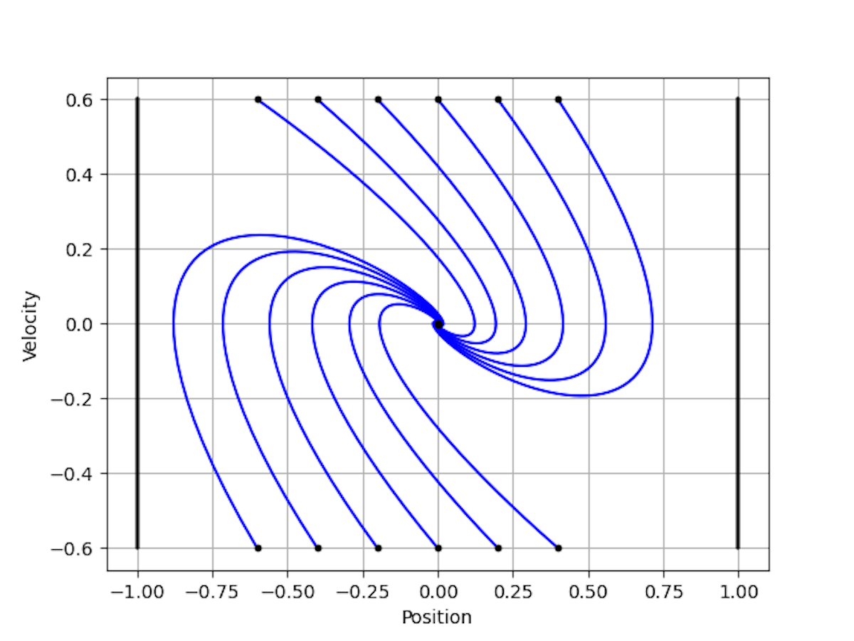
Right here’s a plot of the closed loop from a bunch of preliminary states.

MPC closed loop from varied preliminary states. Picture by writer.

4. Additional subjects

4.1 Stability and Recursive Feasibility

Two of crucial facets of an MPC controller are recursive feasibility of the iteratively invoked OCP and stability of the closed loop. In different phrases, if I’ve solved the OCP at time (ok), will there exist an answer to the OCP at time (ok+1)? If there exists an answer to the OCP at each time step, will the closed-loop state asymptotically settle at an equilibrium level (i.e. will it’s secure)?

Guaranteeing that an MPC controller reveals these two properties includes fastidiously designing the associated fee operate and constraints, and selecting an extended sufficient prediction horizon. Going again to our instance, recall that the matrices in the associated fee operate had been merely chosen to be:

[
Q = left( begin{array}{cc}
1 & 0
0 & 1
end{array}
right),, Q_K = left( begin{array}{cc}
1 & 0
0 & 1
end{array}
right),, R = 1.
]

In different phrases, the OCP penalises the space of the state to the origin and thus drives it there. As you possibly can in all probability guess, if the prediction horizon, (Ok), may be very brief and the preliminary state is positioned very near the constraints at (x_1=pm 1), the OCP will discover options with inadequate “foresight” and the issue can be infeasible at some future iteration of the MPC loop. (You can too experiment with this by making (Ok) small within the code.)

4.2 Some Different Subjects

MPC is an energetic subject of analysis and there are various fascinating subjects to discover.

What if the total state can’t be measured? This pertains to observability and output MPC. What if I don’t care about asymptotic stability? This (typically) has to do with financial MPC. How do I make the controller strong to noise and disturbances? There are just a few methods to cope with this, with tube MPC in all probability being the best-known.

Future articles would possibly give attention to a few of these subjects.