Understanding Matrices | Half 2: Matrix-Matrix Multiplication

Why Open Supply is No Longer Non-compulsory — And Find out how to Make it Work for Your Enterprise

A Sensible Starters’ Information to Causal Construction Studying with Bayesian Strategies in Python

Within the first story [1] of this sequence, we’ve got:

Addressed multiplication of a matrix by a vector,
Launched the idea of X-diagram for a given matrix,
Noticed conduct of a number of particular matrices, when being multiplied by a vector.

Within the present 2nd story, we’ll grasp the bodily which means of matrix-matrix multiplication, perceive why multiplication isn’t a symmetrical operation (i.e., why “A*B ≠ B*A“), and at last, we’ll see how a number of particular matrices behave when being multiplied over one another.

So let’s begin, and we’ll do it by recalling the definitions that I exploit all through this sequence:

Matrices are denoted with uppercase (like ‘A‘ and ‘B‘), whereas vectors and scalars are denoted with lowercase (like ‘x‘, ‘y‘ or ‘m‘, ‘n‘).
|x| – is the size of vector ‘x‘,
rows(A) – variety of rows of matrix ‘A‘,
columns(A) – variety of columns of matrix ‘A‘.

The idea of multiplying matrices

Multiplication of two matrices “A” and “B” might be the commonest operation in matrix evaluation. A identified truth is that “A” and “B” could be multiplied provided that “columns(A) = rows(B)”. On the similar time, “A” can have any variety of rows, and “B” can have any variety of columns. Cells of the product matrix “C = A*B” are calculated by the next system:

[
begin{equation*}
c_{i,j} = sum_{k=1}^{p} a_{i,k}*b_{k,j}
end{equation*}
]

the place “p = columns(A) = rows(B)”. The outcome matrix “C” may have the size:

rows(C) = rows(A),
columns(C) = columns(B).

Performing upon the multiplication system, when calculating “A*B” we should always scan i-th row of “A” in parallel to scanning j-th column of “B“, and after summing up all of the merchandise “a_i,ok*b_ok,j” we may have the worth of “c_i,j“.

The row and the column that needs to be scanned, to calculate cell “c_i,j” of the product matrix “C = A*B”. Right here we scan the third row of “A” and the 2nd column of “B”, by which we acquire the worth “c_3,2“.

One other well-known truth is that matrix multiplication isn’t a symmetrical operation, i.e., “A*B ≠ B*A“. With out going into particulars, we are able to already see that when multiplying 2 rectangular matrices:

Two matrices “A” and “B”, with sizes 2×4 and 4×2, respectively. Multiplying “A*B” will lead to a 2×2-sized matrix, whereas multiplying “B*A” will lead to a 4×4-sized matrix. The highlighted areas present instructions of scans – crimson areas for calculating one cell of “A*B”, and inexperienced areas for calculating a cell of “B*A”.

For newbies, the truth that matrix multiplication isn’t a symmetrical operation usually appears unusual, as multiplication outlined for nearly another object is a symmetrical operation. One other truth that’s usually unclear is why matrix multiplication is carried out by such an odd system.

On this story, I’m going to present my solutions to each of those questions, and never solely to them…

Derivation of the matrices multiplication system

Multiplying “A*B” ought to produce such a matrix ‘C‘, that:

y = C*x = (A*B)*x = A*(B*x).

In different phrases, multiplying any vector ‘x‘ by the product matrix “C=A*B” ought to lead to the identical vector ‘y‘, which we’ll obtain if at first multiplying ‘B‘ by ‘x‘, after which multiplying ‘A‘ by that intermediate outcome.

This already explains why in “C=A*B“, the situation that “columns(A) = rows(B)” needs to be saved. That’s due to the size of the intermediate vector. Let’s denote it as ‘t‘:

t = B*x,
y = C*x = (A*B)*x = A*(B*x) = A*t.

Clearly, as “t = B*x“, we’ll obtain a vector ‘t‘ of size “|t| = rows(B)”. However later, matrix ‘A‘ goes to be multiplied by ‘t‘, which requires ‘t‘ to have the size “|t| = columns(A)”. From these 2 info, we are able to already determine that:

rows(B) = |t| = columns(A), or
rows(B) = columns(A).

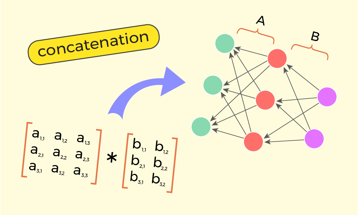
Within the first story [1] of this sequence, we’ve got discovered the “X-way interpretation” of matrix-vector multiplication “A*x“. Contemplating that for “y = (A*B)x“, vector ‘x‘ goes at first by the transformation of matrix ‘B‘, after which it continues by the transformation of matrix ‘A‘, we are able to broaden the idea of “X-way interpretation” and current matrix-matrix multiplication “A*B” as 2 adjoining X-diagrams:

The transformation of vector ‘x’ (the appropriate stack), passing by the product matrix “C=A*B”, from proper to left. At first, it passes by matrix ‘B’, and an intermediate vector ‘t’ is produced (the center stack). Then ‘t’ passes by the transformation of ‘A’ and the ultimate vector ‘y’ is produced (the left stack).

Now, what ought to a sure cell “c_i,j” of matrix ‘C‘ be equal to? From half 1 – “matrix-vector multiplication” [1], we do not forget that the bodily which means of “c_i,j” is – how a lot the enter worth ‘x_j‘ impacts the output worth ‘y_i‘. Contemplating the image above, let’s see how some enter worth ‘x_j‘ can have an effect on another output worth ‘y_i‘. It might probably have an effect on by the intermediate worth ‘t₁‘, i.e., by arrows “a_i,1” and “b_1,j“. Additionally, the love can happen by the intermediate worth ‘t₂‘, i.e., by arrows “a_i,2” and “b_2,j“. Usually, the love of ‘x_j‘ on ‘y_i‘ can happen by any worth ‘t_ok‘ of the intermediate vector ‘t‘, i.e., by arrows “a_i,ok” and “b_ok,j“.

Illustration of all attainable methods through which the enter worth ‘x₂‘ can affect the output worth ‘y₃‘. The affect can undergo intermediate worth ‘t₁‘ (as “a_3,1*b_1,2“), in addition to by intermediate worth ‘t₂‘ (as “a_3,2*b_2,2“), or another k-th worth of the intermediate vector ‘t’ (as “a_3,ok*b_ok,2“). All 4 attainable methods are highlighted right here in crimson.

So there are ‘p‘ attainable methods through which the worth ‘x_j‘ influences ‘y_i‘, the place ‘p‘ is the size of the intermediate vector: “p = |t| = |B*x|”. The influences are:

[begin{equation*}
begin{matrix}
a_{i,1}*b_{1,j},
a_{i,2}*b_{2,j},
a_{i,3}*b_{3,j},
dots
a_{i,p}*b_{p,j}
end{matrix}
end{equation*}]

All these ‘p‘ influences are impartial of one another, which is why within the system of matrices multiplication they take part as a sum:

[begin{equation*}
c_{i,j} =
a_{i,1}*b_{1,j} + a_{i,2}*b_{2,j} + dots + a_{i,p}*b_{p,j} =
sum_{k=1}^{p} a_{i,k}*b_{k,j}
end{equation*}]

That is my visible rationalization of the matrix-matrix multiplication system. By the way in which, deciphering “A*B” as a concatenation of X-diagrams of “A” and “B” explicitly exhibits why the situation “columns(A) = rows(B)” needs to be held. That’s easy, as a result of in any other case it won’t be attainable to concatenate the 2 X-diagrams:

*Making an attempt to multiply such two matrices “C” and “D”, the place “columns(C) ≠ rows(D)”. Their X-diagrams will simply not match one another, and might’t be concatenated.*

Why is it that “AB ≠ BA”

Decoding matrix multiplication “A*B” as a concatenation of X-diagrams of “A” and “B” additionally explains why multiplication isn’t symmetrical for matrices, i.e., why “A*B ≠ B*A“. Let me present that on two sure matrices:

[begin{equation*}
A =
begin{bmatrix}
0 & 0 & 0 & 0
0 & 0 & 0 & 0
a_{3,1} & a_{3,2} & a_{3,3} & a_{3,4}
a_{4,1} & a_{4,2} & a_{4,3} & a_{4,4}
end{bmatrix}
, B =
begin{bmatrix}
b_{1,1} & b_{1,2} & 0 & 0
b_{2,1} & b_{2,2} & 0 & 0
b_{3,1} & b_{3,2} & 0 & 0
b_{4,1} & b_{4,2} & 0 & 0
end{bmatrix}
end{equation*}]

Right here, matrix ‘A‘ has its higher half full of zeroes, whereas ‘B‘ has zeroes on its proper half. Corresponding X-diagrams are:

The X-diagrams which correspond to the matrices “A” and “B” talked about above. Observe, for the zero-cells, we simply don’t draw corresponding arrows.
The truth that ‘A’ has zeroes on its higher rows ends in the higher objects of its left stack being disconnected.
The truth that ‘B’ has zeroes on its proper columns ends in the decrease objects of its proper stack being disconnected.

What’s going to occur if making an attempt to multiply “A*B“? Then A’s X-diagram needs to be positioned to the left of B’s X-diagram.

*Concatenation of X-diagrams of “A” and “B”, equivalent to “A*B”. There are 4 pairs of left and proper objects, which truly can affect one another. An instance pair (y*₃*, x*₁*) is highlighted.*

Having such a placement, we see that enter values ‘x₁‘ and ‘x₂‘ can have an effect on each output values ‘y₃‘ and ‘y₄‘. Notably, which means that the product matrix “A*B” is non-zero.

[
begin{equation*}
A*B =
begin{bmatrix}
0 & 0 & 0 & 0
0 & 0 & 0 & 0
c_{3,1} & c_{3,2} & 0 & 0
c_{4,1} & c_{4,2} & 0 & 0
end{bmatrix}
end{equation*}
]

Now, what is going to occur if we attempt to multiply these two matrices within the reverse order? For presenting the product “B*A“, B’s X-diagram needs to be drawn to the left of A’s diagram:

Concatenation of X-diagrams of “B” and “A”, which corresponds to the product “B*A”. This ends in two disjoint elements, so there isn’t any means through which any merchandise ‘x_j‘ of the appropriate stack can affect any merchandise ‘y_i‘ of the left stack.

We see that now there isn’t any related path, by which any enter worth “x_j” can have an effect on any output worth “y_i“. In different phrases, within the product matrix “B*A” there isn’t any affection in any respect, and it’s truly a zero-matrix.

[begin{equation*}
B*A =
begin{bmatrix}
0 & 0 & 0 & 0
0 & 0 & 0 & 0
0 & 0 & 0 & 0
0 & 0 & 0 & 0
end{bmatrix}
end{equation*}]

This instance clearly illustrates why order is essential for matrix-matrix multiplication. After all, many different examples will also be discovered.

Multiplying chain of matrices

X-diagrams will also be concatenated after we multiply 3 or extra matrices. For example, for the case of:

G = A*B*C,

we are able to draw the concatenation within the following means:

Concatenation of three X-diagrams, equivalent to matrices “A”, “B”, and “C”. Sizes of the matrices are 4×3, 3×2, and a couple of×4, respectively. The two intermediate vectors ‘t’ and ‘s’ are introduced with mild inexperienced and teal objects.

Right here we now have 2 intermediate vectors:

t = C*x, and
s = (B*C)*x = B*(C*x) = B*t

whereas the outcome vector is:

y = (A*B*C)*x = A*(B*(C*x)) = A*(B*t) = A*s.

The variety of attainable methods through which some enter worth “x_j” can have an effect on some output worth “y_i” grows right here by an order of magnitude.

*Two of six attainable methods, highlighted with crimson and light-weight blue, by which enter worth “x₁” can affect output worth “y₃“.*

Extra exactly, the affect of sure “x_j” over “y_i” can come by any merchandise of the primary intermediate stack “t“, and any merchandise of the second intermediate stack “s“. So the variety of methods of affect turns into “|t|*|s|”, and the system for “g_i,j” turns into:

[begin{equation*}
g_{i,j} = sum_{v=1}^s sum_{u=1}^ a_{i,v}*b_{v,u}*c_{u,j}
end{equation*}]

Multiplying matrices of particular sorts

We will already visually interpret matrix-matrix multiplication. Within the first story of this sequence [1], we additionally discovered about a number of particular varieties of matrices – the dimensions matrix, shift matrix, permutation matrix, and others. So let’s check out how multiplication works for these varieties of matrices.

Multiplication of scale matrices

A scale matrix has non-zero values solely on its diagonal:

*The X-diagram of a 4×4 scale matrix. Each enter merchandise “x_i” can have an effect on solely the corresponding output merchandise “y_i“.*

From concept, we all know that multiplying two scale matrices ends in one other scale matrix. Why is it that means? Let’s concatenate X-diagrams of two scale matrices:

*Multiplication of two scale matrices “Q” and “S”, as a concatenation of their X-diagrams.*

The concatenation X-diagram clearly exhibits that any enter merchandise “x_i” can nonetheless have an effect on solely the corresponding output merchandise “y_i“. It has no means of influencing another output merchandise. Due to this fact, the outcome construction behaves the identical means as another scale matrix.

Multiplication of shift matrices

A shift matrix is one which, when multiplied over some enter vector ‘x‘, shifts upwards or downwards values of ‘x‘ by some ‘ok‘ positions, filling the emptied slots with zeroes. To attain that, a shift matrix ‘V‘ should have 1(s) on a line parallel to its essential diagonal, and 0(s) in any respect different cells.

*Instance of a shift matrix ‘V’ and its X-diagram. The matrix shifts upwards all values of the enter vector ‘x’ by 2 positions.*

The idea says that multiplying 2 shift matrices ‘V1‘ and ‘V2‘ ends in one other shift matrix. Interpretation with X-diagrams offers a transparent rationalization of that. Multiplying the shift matrices ‘V1‘ and ‘V2‘ corresponds to concatenating their X-diagrams:

The concatenation of X-diagrams of two shift matrices ‘V1’ and ‘V2’ behaves like one other shift matrix, as each worth of the enter vector ‘x’ continues to be being shifted by a sure variety of positions upwards.

We see that if shift matrix ‘V1‘ shifts values of its enter vector by ‘k1‘ positions upwards, and shift matrix ‘V2‘ shifts values of the enter vector by ‘k2‘ positions upwards, then the outcomes matrix “V3 = V1*V2” will shift values of the enter vector by ‘k1+k2‘ positions upwards, which signifies that “V3” can also be a shift matrix.

Multiplication of permutation matrices

A permutation matrix is one which, when multiplied by an enter vector ‘x‘, rearranges the order of values in ‘x‘. To behave like that, the NxN-sized permutation matrix ‘P‘ should fulfill the next standards:

it ought to have N 1(s),
no two 1(s) needs to be on the identical row or the identical column,
all remaining cells needs to be 0(s).

*An instance of a 5×5-sized permutation matrix ‘P’, and corresponding X-diagram. We see that values of enter vector “(x1, x2, x3, x4, x5)” are being rearranged as “(x4, x1, x5, x3, x2)”.*

Upon concept, multiplying 2 permutation matrices ‘P1‘ and ‘P2‘ ends in one other permutation matrix ‘P3‘. Whereas the explanation for this may not be clear sufficient if matrix multiplication within the extraordinary means (as scanning rows of ‘P1‘ and columns of ‘P2‘), it turns into a lot clearer if it by the interpretation of X-diagrams. Multiplying “P1*P2” is similar as concatenating X-diagrams of ‘P1‘ and ‘P2‘.

*The concatenation of X-diagrams of permutation matrices ‘P1’ and ‘P2’ behaves as one other rearrangement of values.*

We see that each enter worth ‘x_j‘ of the appropriate stack nonetheless has just one path for reaching another place ‘y_i‘ on the left stack. So “P1*P2” nonetheless acts as a rearrangement of all values of the enter vector ‘x‘, in different phrases, “P1*P2” can also be a permutation matrix.

Multiplication of triangular matrices

A triangular matrix has all zeroes both above or under its essential diagonal. Right here, let’s think about upper-triangular matrices, the place zeroes are under the principle diagonal. The case of lower-triangular matrices is comparable.

*Instance of an upper-triangular matrix ‘B’ and its X-diagram.*

The truth that non-zero values of ‘B‘ are both on its essential diagonal or above, makes all of the arrows of its X-diagram both horizontal or directed upwards. This, in flip, signifies that any enter worth ‘x_j‘ of the appropriate stack can have an effect on solely these output values ‘y_i‘ of the left stack, which have a lesser or equal index (i.e., “i ≤ j“). That is among the properties of an upper-triangular matrix.

In accordance with concept, multiplying two upper-triangular matrices ends in one other upper-triangular matrix. And right here too, interpretation with X-diagrams supplies a transparent rationalization of that truth. Multiplying two upper-triangular matrices ‘A‘ and ‘B‘ is similar as concatenating their X-diagrams:

*Concatenation of X-diagrams of two upper-triangular matrices ‘A’ and ‘B’.*

We see that placing two X-diagrams of triangular matrices ‘A‘ and ‘B‘ close to one another ends in such a diagram, the place each enter worth ‘x_j‘ of the appropriate stack nonetheless can have an effect on solely these output values ‘y_i‘ of the left stack, that are both on its stage or above it (in different phrases, “i ≤ j“). Which means that the product “A*B” additionally behaves like an upper-triangular matrix; thus, it should have zeroes under its essential diagonal.

Conclusion

Within the present 2nd story of this sequence, we noticed how matrix-matrix multiplication could be introduced visually, with the assistance of so-called “X-diagrams”. We now have discovered that doing multiplication “C = A*B” is similar as concatenating X-diagrams of these two matrices. This methodology clearly illustrates numerous properties of matrix multiplications, like why it isn’t a symmetrical operation (“A*B ≠ B*A“), in addition to explains the system:

[begin{equation*}
c_{i,j} = sum_{k=1}^{p} a_{i,k}*b_{k,j}
end{equation*}]

We now have additionally noticed why multiplication behaves in sure methods when operands are matrices of particular sorts (scale, shift, permutation, and triangular matrices).

I hope you loved studying this story!

Within the coming story, we’ll deal with how matrix transposition “A^T” could be interpreted with X-diagrams, and what we are able to acquire from such interpretation, so subscribe to my web page to not miss the updates!

My gratitude to:
– Roza Galstyan, for cautious assessment of the draft ( https://www.linkedin.com/in/roza-galstyan-a54a8b352 )
– Asya Papyan, for the exact design of all of the used illustrations ( https://www.behance.internet/asyapapyan ).

In case you loved studying this story, be at liberty to observe me on LinkedIn, the place, amongst different issues, I may even submit updates ( https://www.linkedin.com/in/tigran-hayrapetyan-cs/ ).

All used photographs, until in any other case famous, are designed by request of the creator.