


Machine Studying for Actual-Time Bidding
The previous few years had been a revolution for the cellular promoting and gaming industries, with the broad adoption of neural networks for promoting duties, together with click on prediction. This migration occurred previous to the success of Massive Language Fashions (LLMs) and different AI improvements, however is constructing on the momentum of this wave. The cellular gaming business is spending billions on Person Acquisition yearly, and high gamers on this area comparable to Applovin have market caps of over $100B. On this submit, we’ll focus on a traditional ML strategy for click on prediction, provide motivations for the migration to deep studying for this activity, present a hands-on instance of the advantages of this strategy utilizing an information set from Kaggle, and element among the enhancements that this strategy offers.
Most giant tech corporations within the AdTech area are probably utilizing deep studying for predicting consumer conduct. Social Media platforms have embraced the migration from basic machine studying (ML) to deep studying, as indicated by this Reddit submit and this LinkedIn submit. Within the cellular gaming area Moloco, Liftoff, and Applovin have all shared particulars on their migration to deep studying or {hardware} acceleration to enhance their consumer acquisition platforms. Most Demand Facet Platforms (DSPs) are actually seeking to leverage neural networks to enhance the worth that their platforms present for cellular consumer acquisition.
We’ll begin by discussing logistic regression as an business normal for predicting consumer actions, focus on among the shortfalls of this strategy, after which showcase deep studying as an answer for click on prediction. We’ll present a deep dive on implementations for each a basic ML pocket book and deep studying pocket book for the duty of predicting if a consumer goes to click on on an advert. We received’t dive into the cutting-edge, however we’ll spotlight the place deep studying offers many advantages.
All photographs on this submit, aside from the header picture, had been created from by the creator within the notebooks linked above. The Kaggle information set that we discover on this submit has the CC0: Public Area license.
One of many aim sorts that DSPs usually present for consumer acquisition is a value per click on mannequin, the place the advertiser is charged every time that the platform serves an impression on a cellular system and the consumer clicks. We’ll concentrate on this aim sort to maintain issues easy, however most advertisers desire aim sorts centered on driving installs or buying customers that may spend cash of their app.
In programmatic bidding, a DSP is built-in with a number of advert exchanges, which give stock for the platform to bid on. Most exchanges use a model of the OpenRTB specification to ship bid requests to DSPs and get again responses in a standardized format. For every advert request from a Provide Facet Platform (SSP), the alternate runs an public sale and the DSP that responds with the very best value wins. The alternate then offers the profitable bid response to the SSP, which can lead to an advert impression on a cellular system.
To ensure that a DSP to combine with an advert alternate, there may be an onboarding course of to guarantee that the DSP can meet the technical necessities of an alternate, which usually requires DSPs to reply to bid requests inside 120 milliseconds. What makes this an enormous problem is that some exchanges present over 1 million bid requests per second, and DSPs are normally integrating with a number of exchanges. For instance, Moloco responds to over 5 million requests per second (QPS) throughout peak capability. Due to the latency necessities and big scale of requests, it’s difficult to make use of machine studying for consumer acquisition inside a DSP, however it’s additionally a requirement in an effort to meet advertiser targets.
With the intention to earn cash as a DSP you want to have the ability to ship advert impressions that meet your advertiser targets, whereas additionally producing web income. To perform this, a DSP must bid lower than the anticipated worth that an impression will ship, whereas additionally bidding excessive sufficient to exceed the bid flooring of a request and win in auctions towards different DSPs. A requirement-side platform is billed per impression proven, which corresponds to a CPM (price per impression) mannequin. If the advertiser aim is a goal price per click on (CPC), then the DSP must translate the CPC worth to a CPM worth for bidding. We are able to do that utilizing machine studying and predicting the probability of a consumer to click on on an impression, which we name p_ctr. We are able to this calculate a bid value as follows:
cpm = target_cpc * p_ctr
bid_price = cpm * bid_shade
We use the probability of a click on occasion to transform from price per click on to price per impression after which apply a bid shade with a worth of lower than 1.0 to guarantee that we’re delivering extra worth for advertisers than we’re paying to the advert alternate for serving the impression.
To ensure that a click on prediction mannequin to carry out properly for programmatic consumer acquisition, we would like a mannequin that has the next properties:
- Massive Bias
We wish a click on mannequin that’s extremely discriminative and capable of differentiate between impressions unlikely to lead to a click on and ones which might be extremely prone to lead to a click on. If a mannequin doesn’t have ample bias, it received’t be capable of compete with different DSPs in auctions. - Effectively Calibrated
We wish the expected and precise conversion charges of the mannequin to align properly for the advert impressions the DSP purchases. This implies we now have a desire for fashions the place the output could be interpreted as a chance of a conversion occurring. Poor calibration will lead to inefficient spending. A pattern calibration plot is proven under. - Quick Analysis
We wish to cut back our compute price when bidding on thousands and thousands of requests per second and have fashions which might be quick to inference. - Parallel Analysis
Ideally, we would like to have the ability to run mannequin inference in parallel to enhance throughput. For a single bid request, a DSP could also be contemplating lots of of campaigns to bid for, and each wants a p_ctr worth.

Many advert tech platforms began with logistic regression for click on prediction, as a result of they work properly for the primary 3 desired properties. Over time, it was found that deep studying fashions may carry out higher than logistic regression on the bias aim, with neural networks being higher at discriminating between click on and no-click impressions. Moreover, neural networks can use batch analysis and align will with the fourth property of parallel analysis.
DSPs had been capable of push logistic regression fashions fairly far, which is what we’ll cowl within the subsequent part, however they do have some boundaries of their utility to consumer acquisition. Deep neural networks (DNN) can overcome a few of these points, however current new challenges of their very own.
Advert Tech corporations have been utilizing logistic regression for greater than a decade for click on prediction. For instance, Fb offered utilizing logit together with different fashions at ADKDD 2014. There are lots of alternative ways of utilizing logistic regression for click on prediction, however I’ll concentrate on a single strategy I labored on up to now referred to as Huge Logistic. The overall concept was to show your entire options into tokens, create combos of tokens to symbolize crosses or function interactions, after which create a listing of tokens that you just use to transform your enter options right into a sparse vector illustration. It’s an strategy the place each function is 1-hot encoded and the entire options are binary, which helps simplify hyperparameter tuning for the clicking mannequin. It’s an strategy that may help numeric, categorical, and many-hot options as inputs.
To find out what this strategy seems like in observe, we’ll present a hands-on instance of coaching a click on prediction mannequin utilizing the CTR In Commercial Kaggle information set. The complete pocket book for function encoding, mannequin coaching and analysis is accessible right here. I used Databricks, PySpark, and MLlib for this pipeline.

The dataset offers a coaching information set with labels and a take a look at information set with out labels. For this train we’ll cut up the coaching file into practice and take a look at teams, in order that we now have labels accessible for all information. We create a 90/10% cut up the place the practice set has 414k information and take a look at has 46k information. The information set has 15 columns, which features a label, 2 columns that we’ll ignore (session_id and user_id) and 12 categorical values that we’ll use as options in our mannequin. A couple of pattern information are proven within the desk above.
Step one we’ll carry out is tokenizing the info set, which is a type of 1-hot encoding. We convert every column to a string worth by concatenating the function title and have worth. For instance, we’d create the next tokens for the primary row within the above desk:
[“product_c”, “campaign_id_359520”, “webpage_id_13787”, ..]
For null values, we use “null” as the worth, e.g. “product_null”. We additionally create all combos of two options, which generates extra tokens:
[“product_c*campaign_id_359520”, “”, “product_c*webpage_id_13787”, “campaign_id_359520*webpage_id_13787”,..]
We use a UDF on the PySpark dataframe to transform the 12 columns right into a vector of strings. The ensuing dataframe contains the token checklist and label, as proven under.

We then create a high tokens checklist, assign an index to every token on this checklist, and use the mapping of token title to token index to encode the info. We restricted our token checklist to values the place we now have at the least 1000 examples, which resulted in roughly 2,500 tokens.

We then apply this token checklist to every document within the information set to transform from the token checklist to a sparse vector illustration. If a document contains the token for an index, the worth is about to 1, and if the token is lacking the worth is about to 0. This ends in an information set that we are able to use with MLlib to coach a logistic regression mannequin.

We cut up the dataset into practice and take a look at teams, match the mannequin on the practice information set, after which remodel the take a look at information set to get predictions.
classifier = LogisticRegression(featuresCol = 'options',
labelCol = 'label', maxIter = 50, regParam = 0.01, elasticNetParam = 0)
lr_model = classifier.match(train_df)
pred_df = lr_model.remodel(test_df).cache()
This course of resulted within the following offline metrics, which we’ll examine to a deep studying mannequin within the subsequent part.
Precise Conv: 0.06890
Predicted Conv: 0.06770
Log Loss: 0.24795
ROC AUC: 0.58808
PR AUC: 0.09054
The AUC metrics don’t look nice, however there isn’t a lot sign within the information set with the options that we explored, and different contributors within the Kaggle competitors typically had decrease ROC metrics. One different limitation of the info set is that the specific values are low cardinality, with solely a small variety of distinct values. This resulted in a low parameter depend, with solely 2,500 options, which restricted the bias of the mannequin.
Logistic regression works nice for click on prediction, however the place we run into challenges is when coping with excessive cardinality options. In cellular advert tech, the writer app, the place the advert is rendered, is a excessive cardinality function, as a result of there are thousands and thousands of potential cellular apps which will render an advert. If we wish to embrace the writer app as a function in our mannequin, and are utilizing 1-hot encoding, we’re going to find yourself with a big parameter depend. That is particularly the case after we carry out function crosses between the writer app and different excessive cardinality options, such because the system mannequin.
I’ve labored with logistic regression click on fashions which have greater than 50 million parameters. At this scale, MLlib’s implementation of logistic regression runs into coaching points, as a result of it densifies the vectors in its coaching loop. To keep away from this bottleneck, I used the Fregata library, which performs gradient descent utilizing the sparse vector instantly in a mannequin averaging technique.
The opposite difficulty with giant click on fashions is mannequin inference. If you happen to embrace too many parameters in your logit mannequin, it might be sluggish to guage, considerably rising your mannequin serving prices.
Deep studying is an effective resolution for click on fashions, as a result of it offers strategies for working effectively with very sparse options with excessive cardinality. One of many key layers that we’ll use in our deep studying mannequin is an embedding layer, which takes a categorical function as an enter and a dense vector as an output. With an embedding layer, we be taught a vector for every of the entries in our vocabulary for a categorical function, and the variety of parameters is the dimensions of the vocabulary occasions the output dense vector measurement, which we are able to management. Neural networks can cut back the parameter depend by creating interactions between the dense layers output of embeddings, moderately than making crosses between the sparse 1-hot encoded strategy utilized in logistic regression.
Embedding layers are only one means that neural networks can present enhancements over logistic regression fashions, as a result of deep studying frameworks present quite a lot of layer sorts and architectures. We’ll concentrate on embeddings for our pattern mannequin to maintain issues simplistic. We’ll create a pipeline for encoding the info set into TensorFlow Data after which practice a mannequin utilizing embeddings and cross layers to carry out click on prediction. The complete pocket book for information preparation, mannequin coaching and analysis is accessible right here.

Step one that we carry out is producing a vocabulary for every of the options that we wish to encode. For every function, we discover all values with greater than 100 cases, and all the pieces else is grouped into an out-of-vocab (OOV) worth. We then encode the entire categorical options and mix them right into a single tensor named int, as proven under.

We then save the Spark dataframe as TensorFlow information to cloud storage.
output_path = "dbfs:/mnt/ben/kaggle/practice/"
train_df.write.format("tfrecords").mode("overwrite").save(output_path)
We then copy the recordsdata to the motive force node and create TensorFlow information units for coaching and evaluating the mannequin.
def getRecords(paths):
options = {
'int': FixedLenFeature([len(vocab_sizes)], tf.int64),
'label': FixedLenFeature([1], tf.int64)
}@tf.operate
def _parse_example(x):
f = tf.io.parse_example(x, options)
return f, f.pop("label")
dataset = tf.information.TFRecordDataset(paths)
dataset = dataset.batch(10000)
dataset = dataset.map(_parse_example)
return dataset
training_data = getRecords(train_paths)
test_data = getRecords(test_paths)
We then create a Keras mannequin, the place the enter layer is an embedding layer per categorical function, we now have two hidden cross layers, and a remaining output layer that could be a sigmoid activation for the propensity prediction.
cat_input = tf.keras.Enter(form=(len(vocab_sizes)),
title = "int", dtype='int64')
input_layers = [cat_input]cross_inputs = []
for attribute in categories_index:
index = categories_index[attribute]
measurement = vocab_sizes[attribute]
category_input = cat_input[:,(index):(index+1)]
embedding = keras.layers.Flatten()
(keras.layers.Embedding(measurement, 5)(category_input))
cross_inputs.append(embedding)
cross_input = keras.layers.Concatenate()(cross_inputs)
cross_layer = tfrs.layers.dcn.Cross()
crossed_ouput = cross_layer(cross_input, cross_input)
cross_layer = tfrs.layers.dcn.Cross()
crossed_ouput = cross_layer(cross_input, crossed_ouput)
sigmoid_output=tf.keras.layers.Dense(1,activation="sigmoid")(crossed_ouput)
mannequin = tf.keras.Mannequin(inputs=input_layers, outputs = [ sigmoid_output ])
mannequin.abstract()
The ensuing mannequin has 7,951 parameters, which is about 3 occasions the dimensions of our logistic regression mannequin. If the classes had bigger cardinalities, then we’d anticipate the parameter depend of the logit mannequin to be greater. We practice the mannequin for 40 epochs:
metrics=[tf.keras.metrics.AUC(), tf.keras.metrics.AUC(curve="PR")]mannequin.compile(optimizer=tf.keras.optimizers.Adam(learning_rate=1e-3),
loss=tf.keras.losses.BinaryCrossentropy(), metrics=metrics)
historical past = mannequin.match(x = training_data, epochs = 40,
validation_data = test_data, verbose=0)
We are able to now examine the offline metrics between our logistic regression and DNN fashions:
                Logit    DNN
Precise Conv:    0.06890  0.06890
Predicted Conv: 0.06770  0.06574
Log Loss:       0.24795  0.24758
ROC AUC:        0.58808  0.59284
PR AUC:         0.09054  0.09249
We do see enhancements to the log loss metric the place decrease is best and the AUC metrics the place greater is best. The primary enchancment is to the precision-recall (PR) AUC metric, which can assist the mannequin carry out higher in auctions. One of many points with the DNN mannequin is that the mannequin calibration is worse, and the DNN common predicted worth is additional off than the logistic regression mannequin. We would want to do a bit extra mannequin tuning to enhance the calibration of the mannequin.
We are actually within the period of deep studying for advert tech and corporations are utilizing quite a lot of architectures to ship advertiser targets for consumer acquisition. On this submit, we confirmed how migrating from logistic regression to a easy neural community with embedding layers can present higher offline metrics for a click on prediction mannequin. Listed here are some extra methods we may leverage deep studying to enhance click on prediction:
- Use Embeddings from Pre-trained Fashions
We are able to use fashions comparable to BERT to transform app retailer descriptions into vectors that we are able to use as enter to the clicking mannequin. - Discover New Architectures
We may discover the DCN and TabTransformer architectures. - Add Non-Tabular Knowledge
We may use img2vec to create enter embeddings from artistic property.
Thanks for studying!


