Easy methods to Make Linear Regression Survive Outliers

A easy mannequin with a critical weak point

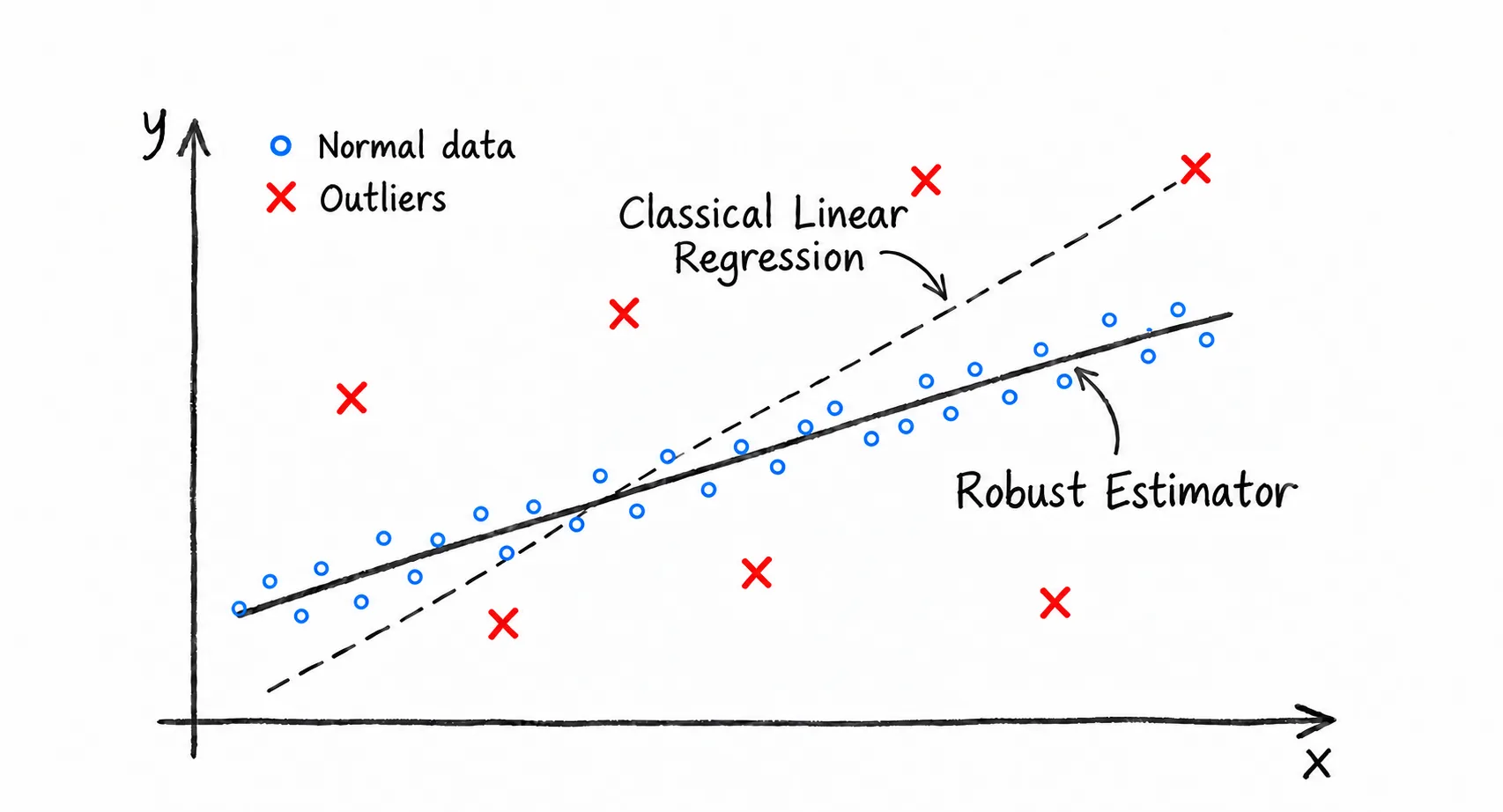
A straight line can look surprisingly convincing—till just a few dangerous measurements pull it someplace it ought to by no means have gone.

Linear regression is usually one of many first predictive fashions practitioners study—and one of many first they put aside when extra refined machine-learning strategies develop into out there. But linear fashions stay beneficial when coefficients want a bodily interpretation, predictions should run on a resource-constrained gadget, computational latency issues, or a easy benchmark is required earlier than introducing a higher-capacity mannequin. They’re additionally helpful as native approximations: even a fancy nonlinear relationship might behave roughly linearly over a small enough area.

Its simplicity, nevertheless, comes with an essential weak point:

Abnormal Least Squares treats each remark as reliable.

In actual knowledge, that assumption is straightforward to violate. A defective sensor, communication error, calibration drawback, or biased measurement can produce observations removed from the connection we really need to estimate. As a result of Abnormal Least Squares (OLS) squares each residual, just a few such observations can have a disproportionate impact. Sturdy estimators attempt to stop these observations from dominating the match.

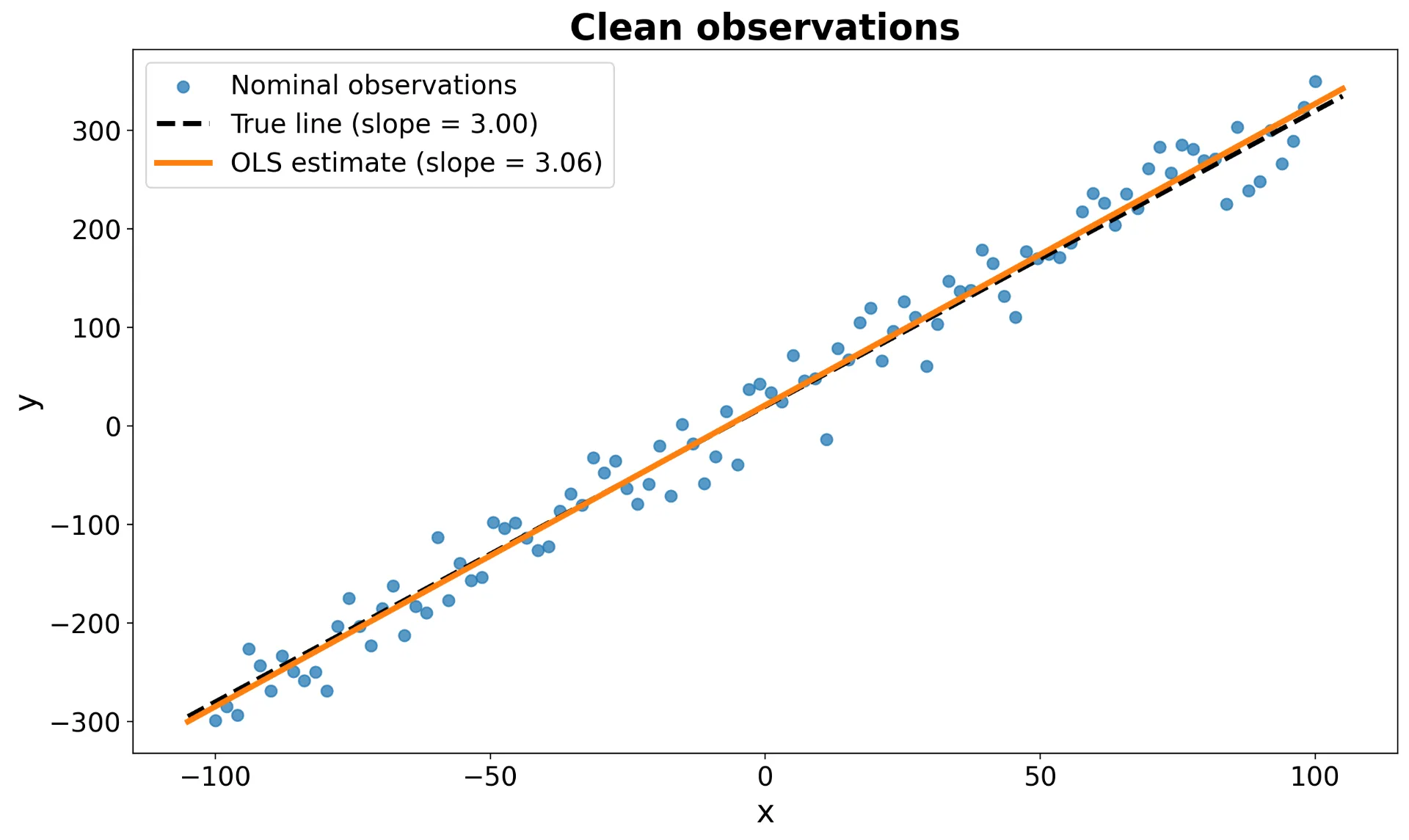
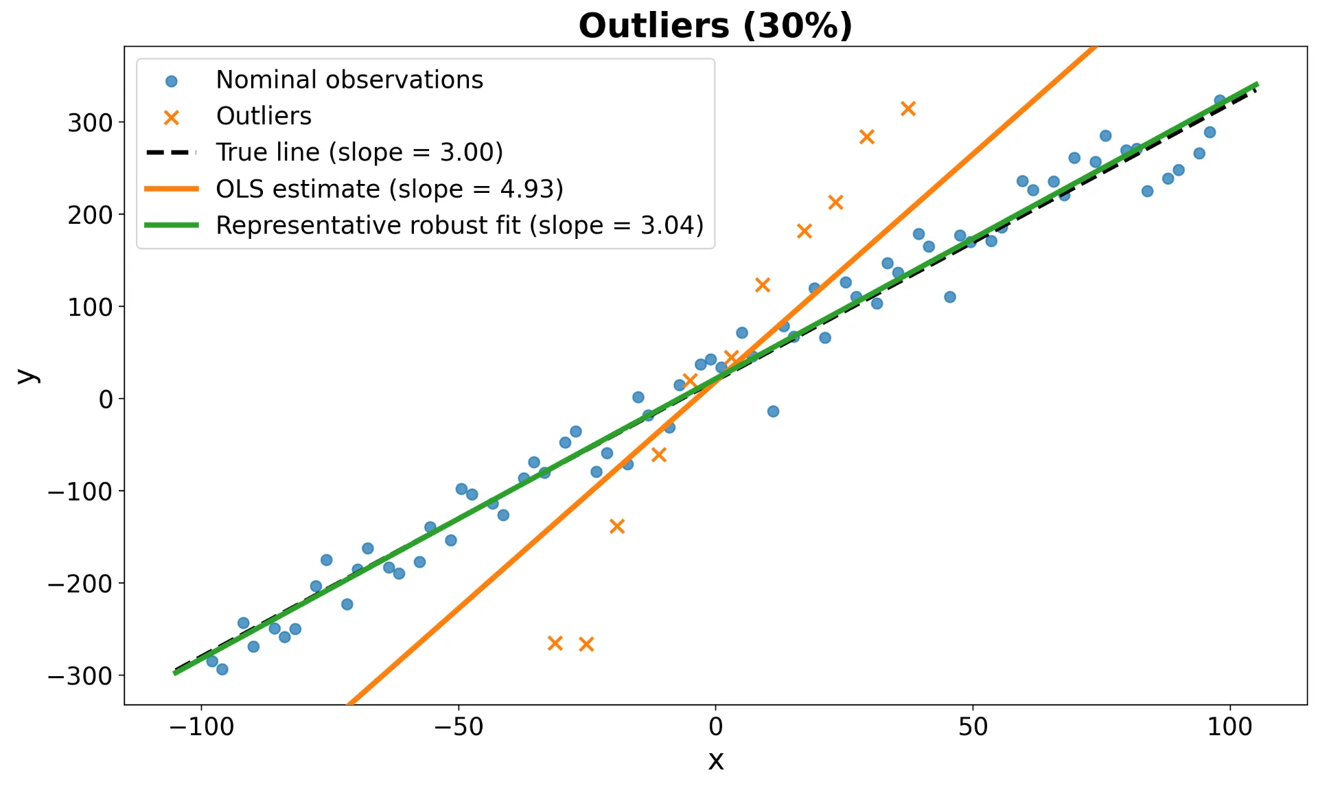
Figures 1 and a couple of present how rapidly the image can change. With clear observations, OLS follows the nominal relationship intently. After 30% of the responses are changed by outliers, the identical estimator is pulled sharply away from it. A consultant strong match, nevertheless, stays a lot nearer to the connection supported by the nominal observations.

That results in the sensible query I need to discover on this article:

How do totally different strong estimators behave once we have no idea the outlier statistics prematurely—and when the contamination turns into progressively more durable?

Realizing {that a} dataset accommodates outliers is simply a part of the issue. In apply, we hardly ever know their proportion, bias, variance, distribution, or construction beforehand. A technique that works effectively for one handy outlier mannequin might behave very in a different way below one other. The estimators listed here are due to this fact examined throughout a number of intentionally totally different types of contamination.

This text compares OLS because the non-robust baseline (Legendre, 1805) with 5 strong estimators: Huber regression (Huber, 1964), Random Pattern Consensus (RANSAC; Fischler and Bolles, 1981), Graduated Non-Convexity with the Geman–McClure loss (GNC-GM), Graduated Non-Convexity with the Truncated Least-Squares loss (GNC-TLS; Yang et al., 2020), and Adaptive Selective Outlier Rejecting (ASOR; Chughtai et al., 2024).

Huber regression and RANSAC are classical robust-estimation strategies, whereas GNC-GM, GNC-TLS, and ASOR signify newer approaches primarily based on non-convex continuation and adaptive residual weighting. Their central algorithmic steps are carried out immediately in order that the weighting, rejection, sampling, stopping, and continuation mechanisms stay seen.

The estimators are evaluated utilizing prediction error and runtime to seize each statistical accuracy and computational effectivity.

Disclosure. The creator developed ASOR within the authentic research cited right here. To make sure a clear comparability, all estimators are evaluated on the identical Monte Carlo realizations utilizing mounted and documented settings.

Why squared loss might be dominated by just a few observations

To see why just a few dangerous measurements can have a lot affect, contemplate the scalar linear mannequin:

Right here, $β₀$

For$N$unbiased observations, maximizing the probability with respect to $β$ is equal to minimizing the OLS goal:

the place

When $boldsymbol{X}$ has full column rank, the acquainted closed-form expression is:

A numerical least-squares solver is preferable to explicitly forming the inverse:

def fit_ols(x, y):    X = np.column_stack((np.ones_like(x), x))    return np.linalg.lstsq(X, y, rcond=None)[0]

The identical squared-loss goal that makes OLS easy and environment friendly additionally creates its fundamental weak point. The contribution of an remark grows quadratically with its residual magnitude:

Thus, a normalized residual of $100$ contributes as a lot to the OLS goal as $10000$ normalized residuals of $1$. A small variety of extreme outliers can due to this fact pull the fitted mannequin away from the connection supported by most observations, as demonstrated in Determine 2.

Sensible observe on lacking values. Rows containing a lacking predictor or response might be excluded earlier than becoming:

legitimate = np.isfinite(X).all(axis=1) & np.isfinite(y)X = X[valid]y = y[valid]

This remedy is suitable when lacking values are restricted and non-systematic. Outliers, nevertheless, are totally different. Lacking observations can often be recognized earlier than becoming, whereas outliers have to be inferred from residuals that rely upon the unknown regression mannequin. Because the fitted mannequin is itself influenced by the outliers, mannequin estimation and outlier identification have to be carried out collectively.

Six estimators, one shared thought

Desk 1. Robustness mechanisms and principal limitations of the six estimators.

A typical method to obtain this joint remedy is to manage the affect of every remark by means of a residual-dependent weight. Most strategies on this comparability due to this fact repeatedly resolve a weighted least-squares drawback:

The sum runs over all $N$observations, and the normalized residual is:

Right here, $w_i$

A shared weighted least-squares engine

Most estimators on this comparability repeatedly resolve the identical weighted least-squares drawback. To maintain their method-specific weighting, sampling, and continuation mechanisms seen, they use the next shared numerical solver:

def weighted_least_squares(x, y, weights=None):    X = np.column_stack((np.ones_like(x), x))    if weights is None:        weights = np.ones(len(y))    sqrt_w = np.sqrt(        np.asarray(weights, dtype=float)    )    Xw = X * sqrt_w[:, None]    yw = np.asarray(y, dtype=float) * sqrt_w    beta, _, rank, _ = np.linalg.lstsq(        Xw, yw, rcond=None    )    if rank < X.form[1]:        elevate np.linalg.LinAlgError(            "Rank-deficient weighted design"        )    return beta

The whole implementations, reproducible pocket book, generated figures, and software program necessities can be found within the public GitHub repository. The repository accommodates the entire weight updates, sampling guidelines, stopping standards, and continuation schedules, whereas the centered snippets introduced right here emphasize the distinguishing operation of every estimator.

OLS: use each remark equally

OLS assigns $w_i=1$

The way it works. Assemble the design matrix, resolve one least-squares drawback, and use all observations at full weight. OLS requires no iterative stopping rule.

def fit_ols(x, y):    return weighted_least_squares(x, y)

OLS is quick, interpretable, and statistically environment friendly when the Gaussian mannequin is suitable. Its limitation is unbounded residual affect: a small variety of extreme observations can transfer the fitted line considerably. For straight-line regression, its price is roughly $mathcal{O}(N)$.

Huber regression: scale back affect easily

OLS fails as a result of each residual receives its full quadratic penalty. The best response isn’t essentially to reject suspicious observations fully, however to scale back how strongly giant residuals can affect the match. Huber regression does precisely that: it’s quadratic for small residuals and linear for giant ones.

The Huber loss is:

Its Iteratively Reweighted Least-Squares replace is:

The way it works. Ranging from OLS, Huber regression computes normalized residuals, assigns unit weight under the edge, reduces the weights above it, and resolves the weighted least-squares drawback. The experiments use $δ = 1.35$

beta = weighted_least_squares(x, y)whereas True:    residuals = (        y - predict(beta, x)    ) / sigma    abs_residuals = np.abs(residuals)    weights = np.minimal(        1.0,        delta / np.most(            abs_residuals,            1e-12,        ),    )    beta_new = weighted_least_squares(        x, y, weights    )    change = (        np.linalg.norm(beta_new - beta)        / max(np.linalg.norm(beta), 1e-12)    )    beta = beta_new    if change <= 1e-5:        break

Huber is a clean and relatively cheap enchancment over OLS. It by no means assigns precisely zero weight, so extreme or systematically biased outliers can proceed to affect the estimate. Its efficiency additionally depends upon the edge. If $I_H$

RANSAC: adaptively seek for a consensus

Huber nonetheless permits each remark to affect the estimate, even when some obtain a lot smaller weights. RANSAC takes a extra aggressive view: as an alternative of softening each giant residual, it searches immediately for a subset of observations that agrees with one mannequin.

For a line, two observations with distinct predictor values outline one mannequin speculation. RANSAC repeatedly samples two observations, evaluates all residuals, and retains the mannequin with the most important inlier consensus. At any time when a bigger consensus is discovered, the estimated inlier fraction is up to date and the required variety of trials is recomputed.

The way it works. Randomly choose an unseen pair of observations, match a candidate line, compute the normalized residuals, and kind a consensus set utilizing a residual threshold. At any time when a bigger consensus is discovered, replace the estimated inlier fraction and recompute the variety of trials required to realize confidence p. This adaptive trial management can terminate the search early when a powerful consensus is recognized. Lastly, refit the mannequin utilizing each remark within the successful consensus set.

The experiments use a normalized residual threshold of $3$ and confidence $p=0.999$

The approximate variety of required hypotheses is:

Right here, $p$ is the specified confidence, $w$ is the estimated inlier fraction, and $s=2$

The ceil operation rounds upward to the closest integer.

total_pairs = math.comb(n, 2)required_trials = total_pairsseen_pairs = set()best_mask = Nonebest_count = 0best_error = np.inftrials = 0whereas (    trials < required_trials    and len(seen_pairs) < total_pairs):    pair = tuple(sorted(        rng.alternative(n, measurement=2, change=False)    ))    if pair in seen_pairs:        proceed    seen_pairs.add(pair)    trials += 1    idx = np.asarray(pair, dtype=int)    beta = weighted_least_squares(        x[idx], y[idx]    )    residuals = np.abs(        y - predict(beta, x)    ) / sigma    masks = residuals <= threshold    depend = int(masks.sum())    error = np.sum(residuals[mask] ** 2)    higher = (        depend > best_count        or (            depend == best_count            and error < best_error        )    )    if higher:        best_mask = masks        best_count = depend        best_error = error        inlier_ratio = best_count / n        success_prob = inlier_ratio ** 2        if success_prob >= 1.0:            required_trials = trials        elif success_prob > 0.0:            adaptive_trials = np.ceil(                np.log1p(-confidence)                / np.log1p(-success_prob)            )            required_trials = min(                required_trials,                max(int(adaptive_trials), trials),            )beta = weighted_least_squares(    x[best_mask], y[best_mask])

RANSAC is efficient when the nominal observations kind a definite and sufficiently giant consensus. Adaptive trial management avoids pointless hypotheses when a powerful consensus is recognized early. Nevertheless, the strategy stays randomized and threshold-dependent, and its price will increase because the inlier fraction decreases. A big coherent outlier cluster also can develop into the successful consensus. For $Okay$ evaluated hypotheses, the approximate price is $mathcal{O}(Okay N)$.

GNC-GM: introduce non-convexity progressively

RANSAC approaches robustness by means of random sampling and consensus. Graduated Non-Convexity (GNC) takes a special route: as an alternative of looking over subsets, it progressively transforms a neater optimization drawback right into a extra strongly strong, non-convex one.

GNC avoids optimizing a strongly non-convex strong loss in a single step. GNC-GM begins with a smoother surrogate and progressively reduces the continuation parameter $mu$. Its weights are:

Following the interpretation of $bar{c}$

The way it works. Initialize with OLS, choose a big $mu$, replace the Geman–McClure weights, and resolve weighted least squares. After every replace, divide $mu$ by $1.4$. The continuation rule stops the process when $mu<1$

beta = weighted_least_squares(x, y)c2 = chi2.ppf(0.99, df=1)residuals = normalized_squared_residuals(    beta, x, y, sigma)mu = 2.0 * residuals.max() / c2whereas mu >= 1.0:    weights = (        (c2 * mu)        / (residuals + c2 * mu)    ) ** 2    beta = weighted_least_squares(        x, y, weights    )    residuals = normalized_squared_residuals(        beta, x, y, sigma    )    mu /= 1.4

The delicate weights make GNC-GM deterministic, comparatively steady, and cheap, however severely biased observations might retain sufficient affect to shift the answer. If $I_{GM}$

GNC-TLS: proceed towards exhausting rejection

GNC-GM reduces the affect of enormous residuals however retains their weights nonzero. GNC-TLS pushes the identical continuation thought additional by progressively transferring towards exhausting rejection by means of the Truncated Least-Squares goal.

For a given $mu$, its weights are:

The way it works. Initialize with OLS and a small continuation parameter, compute the piecewise weights, resolve weighted least squares, and multiply $mu$ by $1.4$ after every replace. The experiments once more select $bar{c}^2$

beta = weighted_least_squares(x, y)c2 = chi2.ppf(0.99, df=1)residuals = normalized_squared_residuals(    beta, x, y, sigma)mu = c2 / max(    2.0 * residuals.max() - c2,    1e-12,)previous_objective = residuals.sum()whereas True:    decrease = (mu / (mu + 1.0)) * c2    higher = ((mu + 1.0) / mu) * c2    weights = np.ones_like(residuals)    weights[residuals >= upper] = 0.0    center = (        (residuals > decrease)        & (residuals < higher)    )    weights[middle] = (        np.sqrt(            c2 * mu * (mu + 1.0)            / residuals[middle]        )        - mu    )    weights = np.clip(weights, 0.0, 1.0)    beta = weighted_least_squares(        x, y, weights    )    residuals = normalized_squared_residuals(        beta, x, y, sigma    )    goal = np.sum(weights * residuals)    change = (        abs(goal - previous_objective)        / max(abs(previous_objective), 1e-12)    )    if change <= 1e-5:        break    previous_objective = goal    mu *= 1.4

This aggressive rejection is helpful below sturdy biased contamination, as a result of sufficiently giant residuals obtain zero weight. It may be computationally costly and depends upon an acceptable inlier threshold. A coherent false construction can nonetheless entice the estimate. If $I_{TLS}$

ASOR: replace probabilistic delicate weights

GNC-GM and GNC-TLS get hold of robustness by means of continuation and residual-dependent weights. ASOR approaches the identical drawback probabilistically. Moderately than instantly deciding whether or not an remark is nominal or corrupted, it estimates how strongly every rationalization is supported by the info and makes use of that proof to find out the remark’s affect on the regression mannequin.

In scalar regression, the load replace is:

Right here, $omega_i$

The posterior nominal-component likelihood and its scaling issue are computed as:

In these expressions, $theta$ is the prior nominal-component likelihood and $Gamma$ denotes the gamma perform. The parameter $b$ controls the outlier-component scale and is up to date collectively with the regression coefficients. Bigger residuals scale back $omega_i$

The way it works. Initialize all weights to at least one, estimate the regression coefficients, compute the normalized squared residuals, replace the posterior nominal-component possibilities, replace the outlier-scale parameter $b$, and kind new probabilistic weights.

The experiments use $a_0=0.5$

weights = np.ones(len(x))b = b0alpha = a0 + 0.5zeta = (    (1.0 / theta - 1.0)    * gamma(alpha)    / gamma(a0))previous_objective = Nonewhereas True:    beta = weighted_least_squares(        x, y, weights    )    residuals = normalized_squared_residuals(        beta, x, y, sigma    )    beta_i = b + 0.5 * residuals    log_term = (        np.log(zeta)        + a0 * np.log(max(b, 1e-12))        - alpha * np.log(            np.most(beta_i, 1e-12)        )        + 0.5 * residuals    )    omega = expit(-log_term)    b = (        prior_a - 1.0        + np.sum(a0 * (1.0 - omega))    ) / (        prior_b        + np.sum(            (1.0 - omega) * alpha / beta_i        )    )    new_weights = (        omega        + (1.0 - omega) * alpha / beta_i    )    goal = np.sum(        new_weights * residuals    )    if previous_objective isn't None:        change = (            abs(goal - previous_objective)            / max(abs(previous_objective), 1e-12)        )        if change <= 1e-5:            break    previous_objective = goal    weights = new_weights

ASOR adaptively balances nominal and outlier explanations with out forcing a right away exhausting choice. Its convergence effort can fluctuate throughout datasets, and its habits depends upon the assumed or estimated nominal-noise scale. A coherent various construction also can entice the estimate. If $I_{mathrm{A}}$

How I stress-tested the estimators

A strong estimator can look spectacular below one handy outlier mannequin and fail badly below one other. Moderately than counting on a single contaminated dataset, I intentionally fluctuate the quantity, distribution, bias, and construction of the corruption.

The nominal relationship all through the experiments is:

The predictor values $x_i$

Impartial substitute outliers

For chosen observations, the nominal error is changed by an outlier error. Gaussian outliers comply with:

Uniform outliers comply with:

The bounds are chosen to match the specified imply and variance:

The outlier statistics are expressed relative to the nominal noise:

Right here, $kappa_{mu}$

sigma_in = np.sqrt(variance_in)nominal_line = 20.0 + 3.0 * xy = nominal_line + rng.regular(    0.0,    sigma_in,    measurement=n,)if distribution == "gaussian":    outlier_noise = rng.regular(        mean_shift_sigma * sigma_in,        np.sqrt(            variance_ratio * variance_in        ),        measurement=n_outliers,    )else:    mean_out = mean_shift_sigma * sigma_in    half_width = np.sqrt(        3.0 * variance_ratio * variance_in    )    outlier_noise = rng.uniform(        mean_out - half_width,        mean_out + half_width,        measurement=n_outliers,    )y[outlier_mask] = (    nominal_line[outlier_mask]    + outlier_noise)

A coherent competing line

Randomly scattered outliers are just one sort of failure. A tougher case seems when the corrupted observations agree with each other and kind a believable various relationship. To check that state of affairs, corrupted observations additionally comply with:

The nominal and competing relationships have the identical intercept and noise variance, however the competing slope is 5 instances bigger. This case exams whether or not an estimator can get well the nominal relationship within the presence of a coherent various construction.

Benchmark design

The experiment households and their fundamental configurations are summarized in Desk 2.

Desk 2. Experiment households and configurations used within the benchmark.

All strategies obtain the identical dataset inside every Monte Carlo realization to make sure a good comparability. All random experiments use deterministic seeds derived from base seed $5000$. Their central algorithmic steps are carried out immediately and evaluated utilizing mounted and documented settings.

The aim is to not declare a common winner from one dataset. I need to see which conclusions survive when the contamination mechanism, pattern measurement, and nominal-noise scale change.

Analysis metrics

I care about two issues: does the strategy get well the proper relationship, and the way a lot computation does that robustness price? Prediction error measures the primary, whereas runtime captures the computational overhead launched by the robustness mechanism.

This overhead issues when giant volumes of high-rate knowledge have to be processed or the mannequin is up to date repeatedly on a resource-constrained gadget. For instance, short-term SNR prediction for GPS jamming detection might require well timed processing of constantly arriving measurements below restricted latency, computing, and vitality budgets, the place extreme computation can scale back battery life. The relative computational prices noticed on this easy regression drawback due to this fact present an early indication of how effectively every estimator might scale in sensible on-line functions.

Every fitted mannequin is evaluated in opposition to the true noiseless relationship on a grid of $J=500$

The sum runs over the J analysis factors. To match experiments throughout totally different nominal-noise scales, the prediction error is normalized as:

Runtime is recorded from one execution of every technique in each Monte Carlo realization and summarized utilizing the median of $30$ measurements in every actual situation, as a result of occasional sluggish executions can distort the imply.

The experiments had been carried out on an HP ProBook 455 G10 geared up with an AMD Ryzen 7 7730U processor—8 cores, 16 logical processors, 2.0 GHz—and 32 GB of RAM, working Microsoft Home windows 11 Professional, Construct 22631.

Absolute execution instances rely upon processor utilization, energy mode, operating-system scheduling, Python and library variations, and the BLAS implementation. The relative ordering and scaling tendencies are due to this fact extra transferable than the precise millisecond values.

Managed assumption. The benchmark provides the true nominal noise scale σᵢₙ to residual-normalized strategies. In apply, this scale could also be calibrated offline from consultant clear measurements. Errors in estimating the nominal noise scale alter the normalized residuals and might due to this fact change threshold-based choices and probabilistic weights. The reported comparability assumes a recognized nominal scale to isolate the habits of the estimators from errors in noise-scale estimation.

What the experiments reveal

As soon as the contamination mechanism adjustments, the relative habits of the estimators adjustments with it. 5 patterns stand out throughout the experiments.

Discovering 1: Biased outliers trigger larger systematic distortion than zero-mean outliers

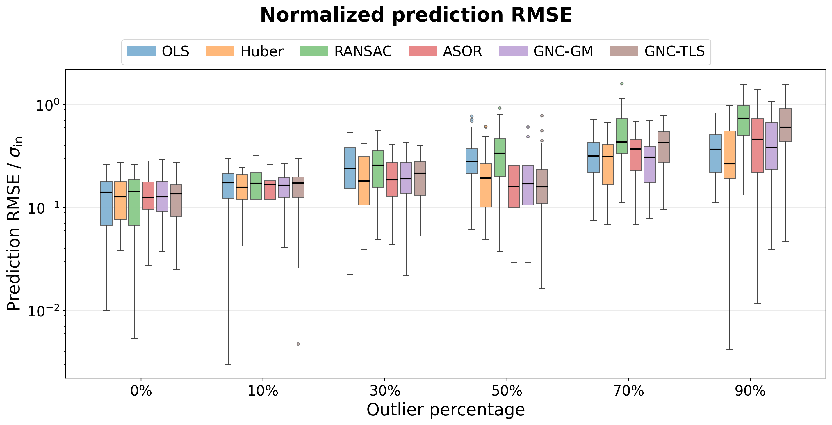
Determine 3 reveals zero-mean Gaussian substitute outliers. Constructive and unfavorable errors partly cancel, so the estimated relationship isn’t constantly pushed in a single path. The strong estimators stay intently matched by means of reasonable contamination, and OLS stays extra correct than it does below biased contamination.

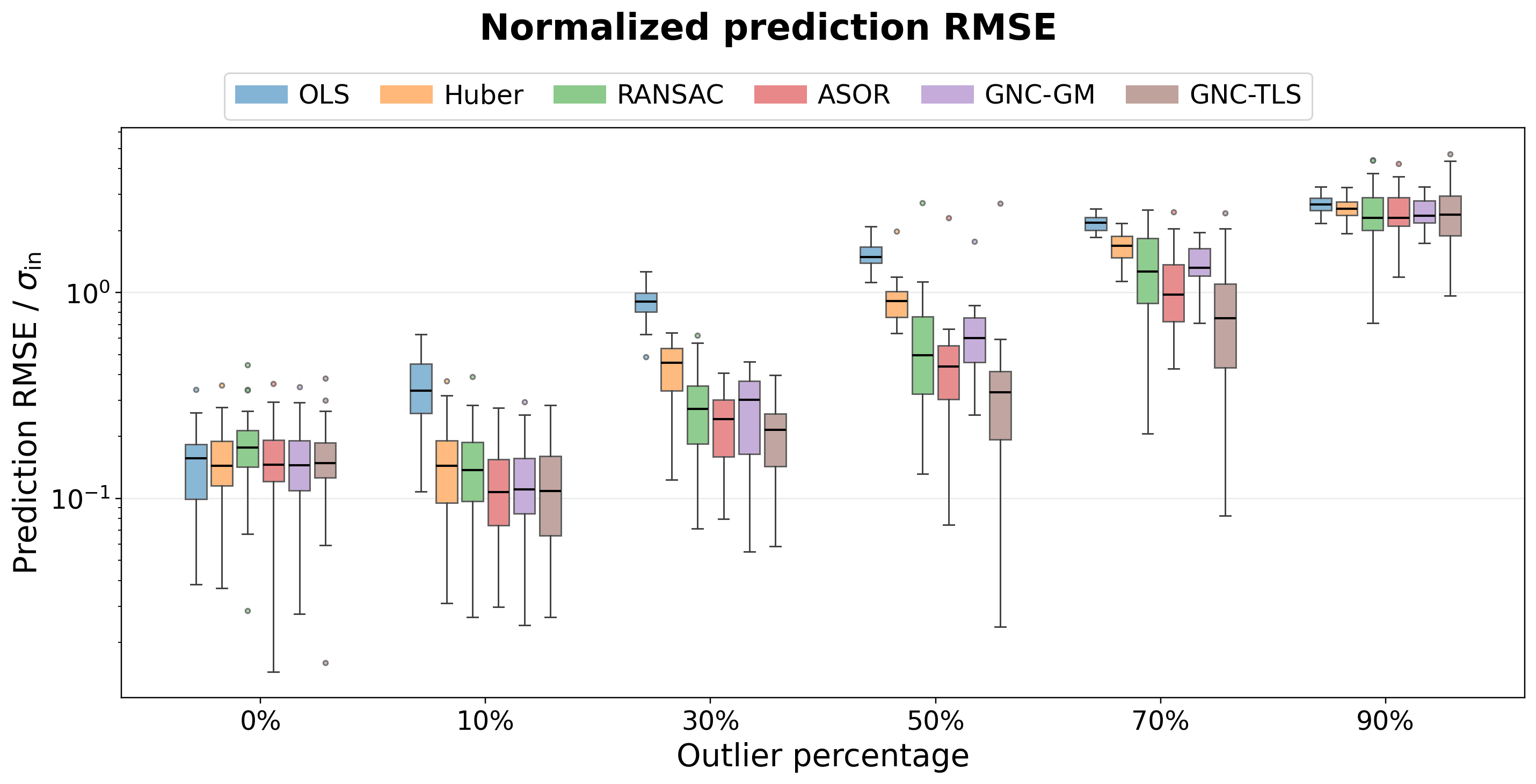
The sample adjustments in Determine 4, the place the outlier imply is shifted by $3sigma_{in}$

The essential distinction is directional consistency. Zero-mean outliers inflate variability, however biased outliers repeatedly pull the slot in the identical path. OLS and Huber are affected most strongly; GNC-TLS and ASOR stay extra correct by means of reasonable contamination. At 90%, the corrupted observations dominate, and the median errors of all six estimators develop into related.

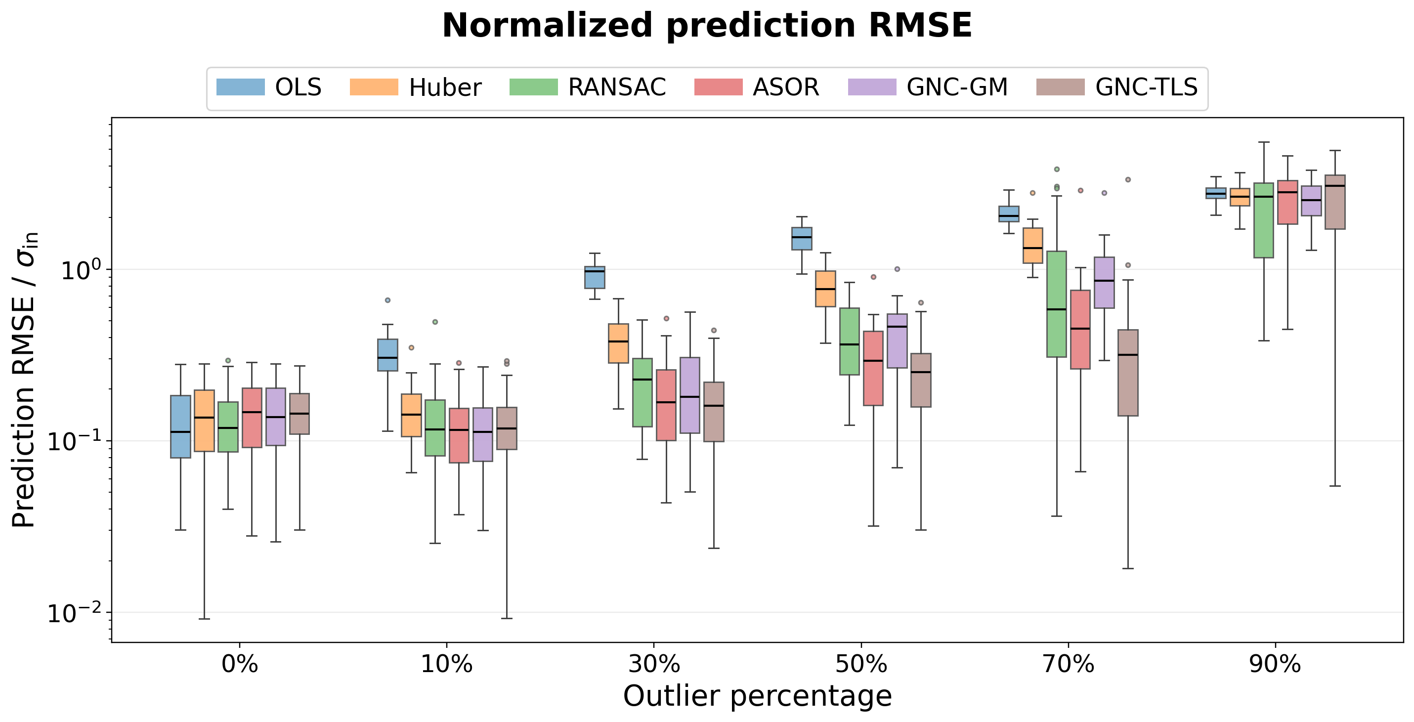
However is that sample particular to Gaussian outliers? To test, Determine 5 repeats the experiment with a biased uniform distribution whose imply and variance are matched to the biased Gaussian case.

The broad rating stays just like the biased Gaussian case. At low outlier percentages, all strong estimators stay comparatively correct as a result of the nominal observations nonetheless dominate the match. As contamination will increase, the variations develop into extra pronounced: GNC-TLS and ASOR preserve the bottom prediction errors by means of reasonable and excessive outlier ranges, whereas OLS and Huber deteriorate extra quickly.

Discovering 2: A coherent competing line is a model-identification drawback

Thus far, the corrupted observations have been unbiased. The following experiment is more durable: what occurs when the outliers themselves kind a coherent various mannequin? Determine 6 evaluates outliers that comply with a second line with 5 instances the nominal slope.

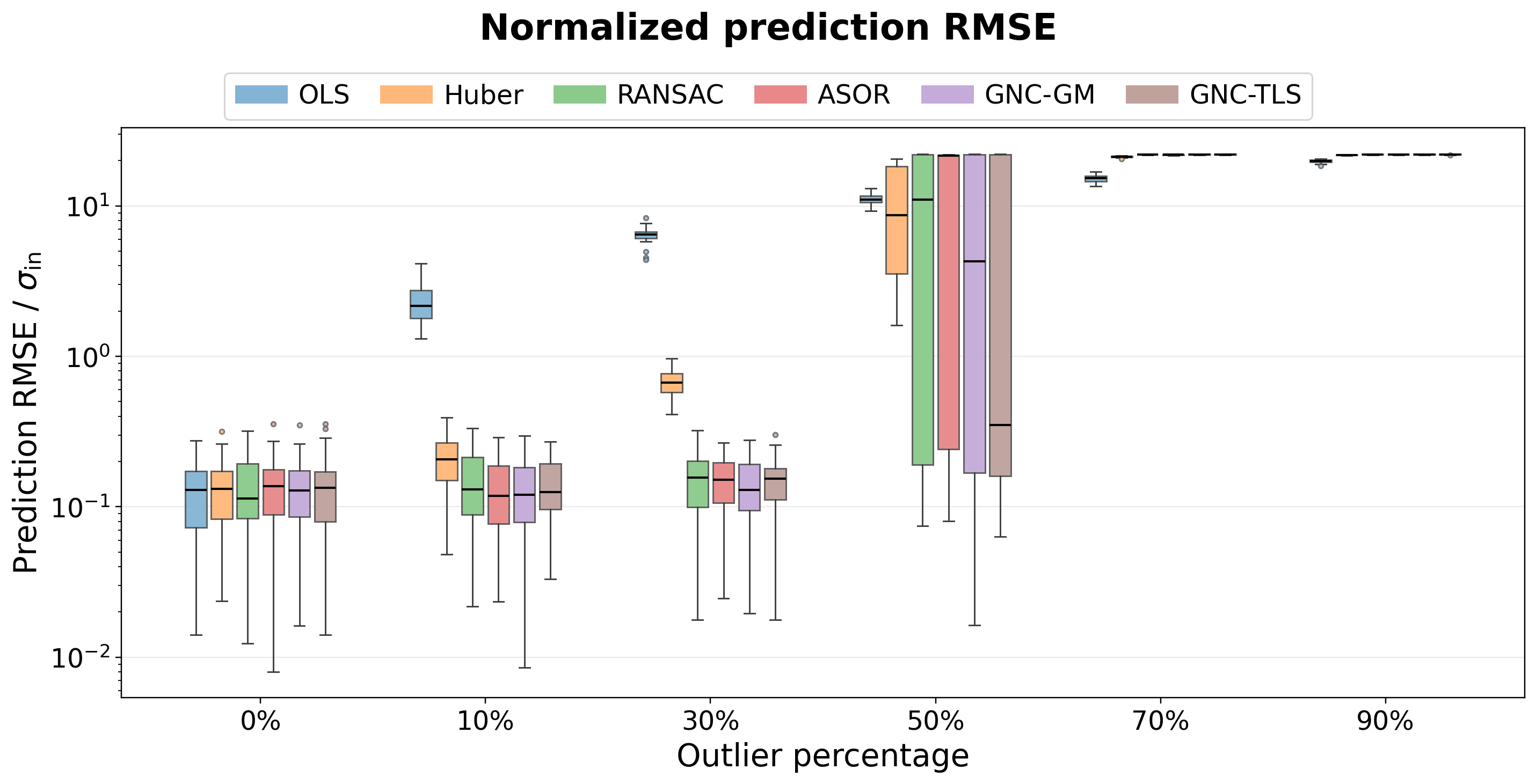
At 10% and 30%, the strong estimators get well the nominal relationship. At 30%, median normalized RMSE values are 0.157 for RANSAC, 0.152 for ASOR, 0.130 for GNC-GM, and 0.154 for GNC-TLS. Huber is much less efficient, whereas OLS is pulled strongly towards the competing line.

The issue turns into basically ambiguous at 50% contamination, the place the nominal and competing constructions comprise the identical variety of observations. The extensive bins point out that totally different Monte Carlo realizations might lead strong estimators towards both of the 2 coherent relationships.

At 70% and 90%, the competing line is the dominant construction. The strong estimators usually choose it, producing normalized RMSE values close to 22 relative to the nominal mannequin. That is an identifiability limitation, not merely a numerical failure. With out labels, bodily constraints, temporal data, or a multi-model formulation, the info alone don’t reveal which coherent relationship is the supposed one.

Discovering 3: Robustness requires extra computation

Accuracy is just one aspect of the story. Robustness requires extra computation, and the strategies pay very totally different costs for it. Determine 7 reveals runtime below biased Gaussian contamination.

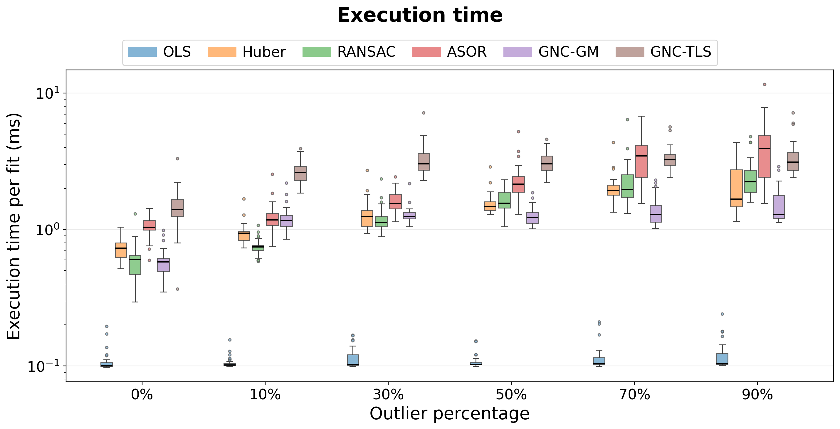
OLS stays quickest as a result of it requires one least-squares resolve. The strong estimators carry out repeated weighted solves or consider a number of RANSAC hypotheses. GNC-GM usually supplies the bottom and most steady iterative price, whereas GNC-TLS is mostly the most costly as a result of its continuation schedule requires extra updates. ASOR occupies an intermediate accuracy–runtime area.

Absolute sub-millisecond timings rely upon the processor, energy mode, operating-system scheduling, Python model, and BLAS implementation. The relative ordering and scaling tendencies are extra transferable than the precise millisecond values.

Desk 3 supplies a consultant comparability throughout all 4 contamination fashions at 50% contamination.

Desk 3. Median execution time in milliseconds at 50% contamination for N = 100 and 30 Monte Carlo realizations.

OLS stays considerably quicker than the strong estimators. Among the many iterative strategies, GNC-GM usually has the bottom and most steady runtime. Huber, RANSAC, and ASOR have intermediate computational prices, whereas GNC-TLS is often the most costly as a result of its continuation schedule requires a number of weighted least-squares solves.

The competing-line case produces an unusually giant Huber runtime at 50% contamination, indicating slower convergence for this specific configuration. This remoted outcome shouldn’t be interpreted as a normal runtime property of Huber regression.

Discovering 4: Extra observations scale back variability, not systematic bias

A pure query is whether or not merely accumulating extra knowledge makes the contamination drawback disappear. Figures 8 and 9 repair biased Gaussian contamination at 50% and fluctuate the pattern measurement from 50 to 5000.

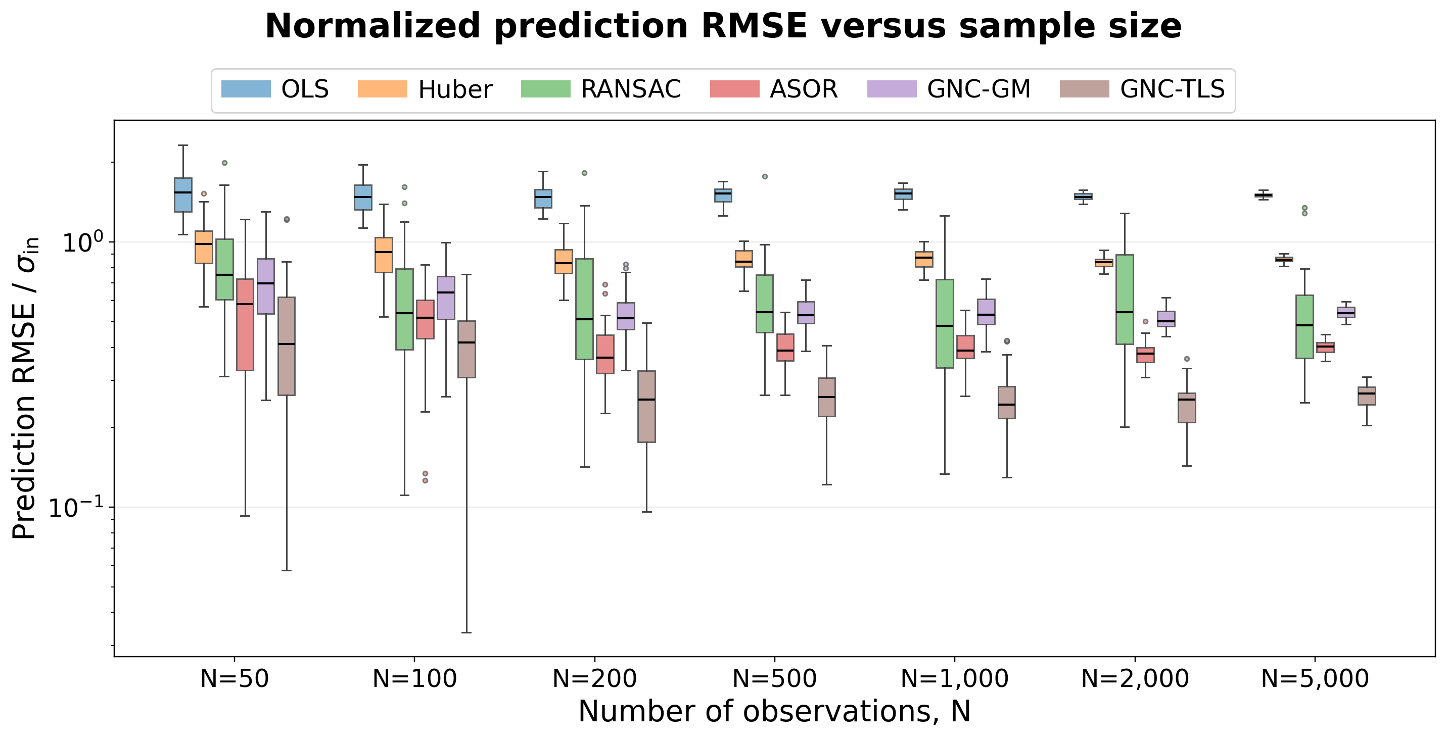
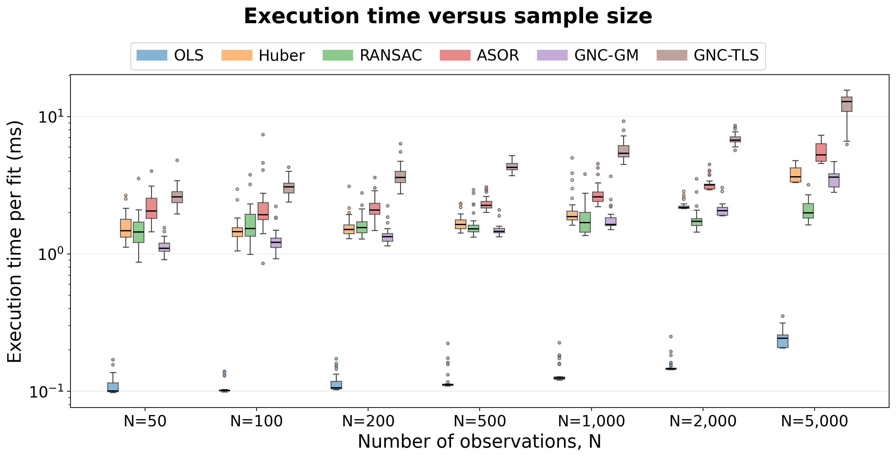
OLS stays biased as N will increase: its median normalized RMSE is 1.533 at $N=50$

GNC-TLS has the bottom median error at each examined pattern measurement. Its median decreases from 0.411 at $N=50$

Runtime will increase with pattern measurement. From $N=50$

RANSAC grows extra slowly as a result of its adaptive stopping rule evaluates the same variety of hypotheses throughout the examined pattern sizes, though every speculation turns into dearer as N will increase.

Discovering 5: Normalization preserves the rating throughout noise scales

Lastly, I modify absolutely the noise scale whereas preserving the relative contamination power. This checks whether or not the noticed rating is tied to at least one specific measurement scale. The ultimate experiment varies:$sigma_{mathrm{in}}^2 in {10, 100, 1000, 10000}$

Desk 4. Median normalized prediction RMSE because the nominal-noise variance adjustments. Boldface marks the 2 lowest values in every column.

The normalized outcomes stay broadly steady as$sigma_{mathrm{in}}^2$

The main strategies stay constant throughout noise scales: GNC-TLS has the bottom median normalized error, adopted by ASOR, whereas OLS has the most important error. The small variations between columns are per finite Monte Carlo variation and present no systematic dependence on absolutely the measurement scale.

Which estimator do you have to begin with?

There isn’t any common winner. The suitable start line depends upon what you already know in regards to the knowledge, how aggressively you might be prepared to reject observations, and the way a lot computation you’ll be able to afford. Area information, residual diagnostics, computational constraints, and sensitivity evaluation ought to all inform the selection. Sensible beginning factors are summarized in Desk 5.

Desk 5. Sensible beginning factors for estimator choice.

The desk is a place to begin, not a choice rule. In apply, I might match multiple strong estimator, examine the ensuing coefficients and residual patterns, and check sensitivity to affordable scale and threshold selections.

Settlement throughout strategies will increase confidence within the recovered relationship; sturdy disagreement is itself helpful proof that the info might comprise a number of constructions or that the assumed nominal-noise scale must be reconsidered.

What this benchmark doesn’t set up

There are additionally clear limits to what these experiments inform us. This can be a managed scalar-regression benchmark, not a common leaderboard for strong estimation. The benchmark research a scalar linear mannequin with one-dimensional residuals, recognized nominal noise, mounted algorithmic settings, and artificial contamination.

Totally different conclusions might emerge for high-dimensional regression, leverage factors within the predictor house, heteroscedastic noise, nonlinear fashions, correlated errors, or actual datasets with unknown floor reality.

The runtime outcomes are implementation- and machine-dependent. The experiments additionally don’t resolve mannequin identification when a number of coherent constructions are current. Sturdy residual weighting can suppress remoted corruption, however it can not decide the supposed mannequin with out extra data as soon as another construction dominates.

What do you have to take away from this?

Essentially the most helpful lesson from these experiments is broader than the rating of the six strategies: the proportion of outliers alone doesn’t decide how troublesome a regression drawback is. Zero-mean outliers can partly cancel, whereas biased observations repeatedly pull the estimate in the identical path. Even Gaussian and uniform outliers with matched first two moments can produce totally different errors. Distribution, bias, and construction all matter.

Extra knowledge assist with variability, however not essentially with bias. When the identical contamination mechanism persists, rising the pattern measurement doesn’t make OLS converge again to the nominal relationship.

In these experiments, GNC-TLS achieved the strongest total accuracy when aggressive rejection was useful, ASOR supplied a positive accuracy–runtime compromise, and GNC-GM supplied comparatively steady computational habits. These rankings are helpful, however they rely upon the assumptions and contamination fashions used right here; they shouldn’t be handled as a common leaderboard.

The competing-line experiment offers the strongest warning. As soon as corrupted observations kind a coherent various relationship, strong regression is now not merely an outlier-rejection drawback. It turns into a model-identification drawback, and residual weighting alone can not inform us which coherent construction is the one we supposed to get well.

Since we hardly ever know precisely how outliers will seem in apply, strong estimators are finest judged throughout a number of believable contamination patterns, with each accuracy and computational price in view.

Subsequent within the sequence. The strong regression sequence continues with polynomial regression, extending the comparability to nonlinear relationships and better mannequin complexity.

References

1. Legendre, A. M. (1805). Nouvelles méthodes pour la détermination des orbites des comètes. F. Didot.

2. Huber, P. J. (1964). Sturdy Estimation of a Location Parameter. The Annals of Mathematical Statistics.

3. Fischler, M. A., and Bolles, R. C. (1981). Random Pattern Consensus: A Paradigm for Mannequin Becoming with Functions to Picture Evaluation and Automated Cartography. Communications of the ACM.

4. Yang, H., Antonante, P., Tzoumas, V., and Carlone, L. (2020). Graduated Non-Convexity for Sturdy Spatial Notion: From Non-Minimal Solvers to World Outlier Rejection. IEEE Robotics and Automation Letters.

5. Chughtai, A. H., Tahir, M., and Uppal, M. (2024). Bayesian Heuristics for Sturdy Spatial Notion. IEEE Transactions on Instrumentation and Measurement.

Get in contact 👋

For extra of my work, discover my GitHub, or join with me on LinkedIn. I welcome questions, new concepts, and alternatives to collaborate in Information science, AI and Statistical Sign Processing. In the event you get pleasure from my articles, sharing them with others helps these conversations attain extra folks.

···

All data-driven figures had been generated by way of simulations by the creator. The featured picture was created with the help of AI.