Reparameterization Tips: Variance Discount by Smarter Gradients

The reparameterization trick is what makes Variational Autoencoders (VAEs) trainable with normal stochastic gradient descent. It really works by shifting randomness exterior the computation graph and turns a clumsy gradient of an expectation into an atypical chain-rule spinoff.

A VAE is a generative mannequin. An encoder maps enter information xto a distribution over a latent variable z, whereas a decoder maps a sampled z again to a reconstruction of x. What makes it trainable is its goal, the ELBO (Proof Decrease Certain) i.e., a tractable stand-in for the true (intractable) information chance, made up of a reconstruction time period and a time period that regularizes the latent distribution towards a easy prior. To coach a VAE entails maximizing this ELBO utilizing gradient descent, and with the intention to try this the gradient of an expectation have to be computed; extra exactly, the gradient of the anticipated reconstruction high quality with respect to randomly sampled latent variables z have to be computed.

It is genuinely awkward to make that distinction and the difficulty shouldn’t be distinctive to VAEs. The identical construction reveals up within the anticipated return in policy-gradient RL, and in variational inference extra usually. In each case we’re optimizing L(θ) = E[f(z)] the place z is itself sampled from a distribution that is determined by θ — so the factor we’re differentiating is outlined by the distribution we’re differentiating with respect to. That circularity is the place a variety of the ache in stochastic optimization comes from, and it is precisely what the reparameterization trick was constructed to sidestep.

This text walks via that drawback, the 2 most important households of gradient estimators used to resolve it, and why the “pathwise” gradients obtained via reparameterization are inclined to have dramatically decrease variance than the choice.

Why low-variance gradients matter in follow

A lower-variance gradient estimator isn’t just a theoretical nicety. In follow, it straight interprets to:

1. Extra steady coaching curves — fewer wild swings within the loss.

2. Sooner convergence — can take bigger efficient steps with much less noise.

3. Higher remaining fashions — the optimizer spends much less time combating gradient noise and extra time becoming the info.

That is particularly crucial for advanced fashions like VAEs, Bayesian neural networks, and continuous-control Reinforcement Studying brokers, the place the coaching sign can in any other case be too noisy to be helpful.

The issue: Gradients of expectations — why sampling breaks backprop

Suppose we wish to optimize

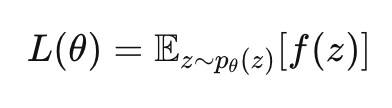
with respect to θ. If θ solely appeared inside f, this could be a typical backprop drawback. The complication is that θ parameterizes the distribution that z is drawn from — the sampling course of itself is determined by θ — so we will not simply push the gradient via a hard and fast computation graph. Monte Carlo estimates of L(θ) are simple (draw samples, common f(z)), however Monte Carlo estimates of ∇θ L(θ) will not be computerized, as a result of differentiating via a sampling operation is not properly outlined.

There are two basic methods out of this: the rating operate estimator (REINFORCE) and the pathwise / reparameterization estimator. Each are unbiased. They differ enormously in variance.

The rating operate estimator (REINFORCE): versatile however excessive variance

The traditional trick right here is the log-derivative identification:

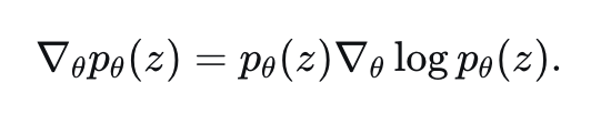
Substituting this into the gradient of the expectation offers

which is now an expectation once more, so it may be estimated by sampling z ~ p_θ and averaging f(z)·∇θ log p_θ(z). That is the estimator behind REINFORCE in policy-gradient reinforcement studying, and it is genuinely versatile. It really works for discrete zand it does not require f to be differentiable in any respect. Solely p_θ wants a tractable, differentiable log-density.

The price of that generality is variance. The estimator solely ever sees the scalar worth f(z). It has no details about how f adjustments as z adjustments. When f(z) is roughly the identical for many sampled z however the rating ∇θ log p_θ(z) fluctuates lots (which it does, particularly in excessive dimensions or with peaked distributions), the product f(z)·rating turns into a loud amount with excessive variance, and that noise reveals up straight within the gradient estimate. Because of this REINFORCE-style estimators nearly all the time want variance-reduction equipment bolted on — baselines, management variates, benefit normalization; to be usable in follow.

The reparameterization trick: pathwise gradients made differentiable

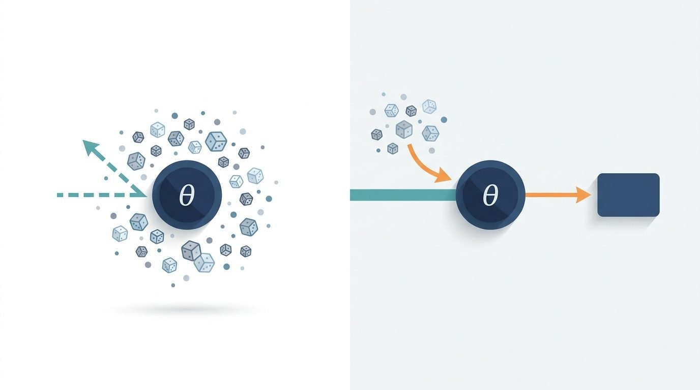
The choice is to alter how we generate z. As an alternative of sampling z straight from p_θ, we specific z as a deterministic, differentiable operate of θ and an auxiliary noise variable ε whose distribution does not depend upon θ:

The canonical instance is the Gaussian: as a substitute of sampling z ~ N(μ, σ²) straight, pattern ε ~ N(0, 1) and set z = μ + σ·ε. All of the randomness now lives in ε, which is fastened and unbiased of θ. θ solely enters via a deterministic transformation.

With that reformulation, the expectation turns into

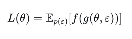
and since the distribution we’re integrating over now not is determined by θ, we are able to push the gradient straight inside:

That is the pathwise spinoff: for every sampled ε, we differentiate f via the deterministic path z = g(θ, ε) utilizing the atypical chain rule, precisely as if we had been backpropagating via some other layer in a neural community. In reality, as soon as z is reparameterized this manner, sampling turns into simply one other differentiable operation within the computation graph, and normal autodiff handles the remaining.

Why reparameterization reduces gradient variance

The intuitive motive pathwise gradients are typically a lot decrease variance is that they really use native, first-order details about f i.e., the spinoff f'(z); whereas the score-function estimator solely ever makes use of the worth f(z). Two samples that land shut collectively in z-space may have comparable pathwise gradient contributions (as a result of f is domestically clean), however they will have wildly completely different score-function contributions, as a result of the rating ∇θ log p_θ(z) does not know something about f and may swing sharply even between close by factors. The pathwise estimator successfully differentiates the reward floor straight. The score-function estimator has to deduce sensitivity to θ not directly, by how a lot roughly probably a given pattern turns into. It is a a lot noisier sign. This comparability is formalized properly in Mohamed et al.’s survey on Monte Carlo gradient estimation, which frames each estimators inside a typical framework and derives circumstances underneath which every has decrease variance.

A numerical instance: rating operate vs reparameterization

Take the toy drawback L(θ) = E[z²], z ~ N(θ, 1), for which the true gradient is solely 2θ. Estimating this gradient two methods: rating operate vs. reparameterization, with the identical variety of samples per estimate:

import numpy as npimport matplotlib.pyplot as pltnp.random.seed(0)theta = 1.5sigma = 1.0true_grad = 2 * thetadef score_function_grad(n):    z = np.random.regular(theta, sigma, dimension=n)    f = z**2    rating = (z - theta) / sigma**2       # d/dtheta log N(z; theta, sigma^2)    return (f * rating).imply()def reparam_grad(n):    eps = np.random.regular(0, 1, dimension=n)    z = theta + sigma * eps    return (2 * z).imply()                # df/dtheta through chain rule, dz/dtheta = 1n = 20sf = np.array([score_function_grad(n) for _ in range(20000)])rp = np.array([reparam_grad(n) for _ in range(20000)])print("true grad:", true_grad)print("score-function  imply/var:", sf.imply(), sf.var())print("reparameterized imply/var:", rp.imply(), rp.var())print("variance ratio (SF / reparam):", sf.var() / rp.var())plt.hist(sf, bins=50, alpha=0.5, label="Rating operate")plt.hist(rp, bins=50, alpha=0.5, label="Reparameterization")plt.axvline(true_grad, colour="okay", linestyle="--", label="True gradient")plt.legend()plt.xlabel("Gradient estimate")plt.ylabel("Frequency")plt.title("Distribution of gradient estimates (n = 20)")plt.present()

Operating this provides each estimators converging to the right gradient (≈3.0) on common, however with

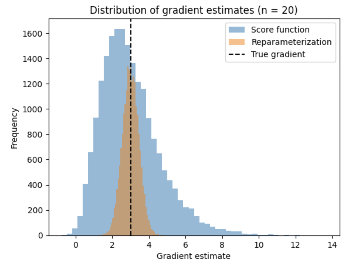
Histogram evaluating the distribution of score-function and reparameterized gradient estimates; the reparameterized estimates cluster tightly across the true gradient.

Roughly a 13x discount in variance from reparameterization alone, on an issue this straightforward. In higher-dimensional, extra peaked posteriors, the regime VAEs and variational inference truly function in, the hole tends to widen additional, which is a giant a part of why reparameterized ELBO estimators made scalable variational inference sensible within the first place.

When can we use the reparameterization trick?

Reparameterization is not free. It requires a differentiable sampling path, which not each distribution has in closed type.

• Location-scale households (Gaussian, Logistic, Laplace, uniform) reparameterize trivially, as above.

• Distributions with a tractable inverse CDF might be reparameterized through inverse-transform sampling: draw u ~ Uniform(0,1) and set z = F_θ⁻¹(u).

• Extra advanced steady distributions (Gamma, Beta, Dirichlet, von Mises) haven’t got a easy location-scale type, however can nonetheless be dealt with via implicit reparameterization gradients, which differentiate via the CDF itself somewhat than requiring an express sampling path (Figurnov et al., 2018).

• Discrete random variables (categorical, Bernoulli) don’t have any differentiable sampling path. Small adjustments in θ do not change z repeatedly. The usual workaround is a steady rest: the Gumbel-Softmax / Concrete distribution replaces the arduous discrete pattern with a temperature-controlled steady approximation that is reparameterizable, buying and selling a small quantity of bias for a reparameterized low-variance gradient (Jang, Gu & Poole, 2016; Maddison, Mnih & Teh, 2016).

• Even inside reparameterizable fashions, additional variance discount is feasible. As an illustration, the “sticking the touchdown” trick removes a score-function time period that leaks again into supposedly pathwise ELBO gradients because the approximate posterior converges to the true one (Roeder, Wu & Duvenaud, 2017).

Reparameterization in follow: VAEs, RL, and variational inference

• Variational autoencoders use reparameterization to get low-variance gradients of the ELBO with respect to the encoder parameters. That is basically what made VAEs trainable with normal SGD (Kingma & Welling, 2013; Rezende, Mohamed & Wierstra, 2014).

• Coverage-gradient reinforcement studying with steady motion areas can use the reparameterized (“pathwise”) coverage gradient as a substitute of REINFORCE, which is likely one of the causes algorithms like Smooth Actor-Critic are comparatively sample-efficient.

• Variational inference extra broadly (Bayesian deep studying, Bayesian neural networks, probabilistic programming) depends on reparameterized gradients to suit approximate posteriors through stochastic optimization as a substitute of MCMC.

Rating operate vs pathwise estimator: abstract

The reparameterization trick shouldn’t be a distinct optimisation algorithm; somewhat, it’s a change of variables that converts ‘differentiating via a sampling course of’ into ‘differentiating via an atypical deterministic operate’, permitting the chain rule to hold out the duty it’s good at. Since such a change is feasible at any time when the underlying distribution permits it, it’s nearly all the time value utilizing as a substitute for a score-function estimator, just because it supplies the optimizer with a a lot cleaner gradient sign.

References

For all of the articles I’ve referenced on this article, you possibly can examine these hyperlinks.

1. Kingma, D. P., & Welling, M. (2013). Auto-Encoding Variational Bayes. arxiv.org/abs/1312.6114

2. Rezende, D. J., Mohamed, S., & Wierstra, D. (2014). Stochastic Backpropagation and Approximate Inference in Deep Generative Fashions. arxiv.org/abs/1401.4082

3. Mohamed, S., Rosca, M., Figurnov, M., & Mnih, A. (2020). Monte Carlo Gradient Estimation in Machine Studying. Journal of Machine Studying Analysis. jmlr.org/papers/v21/19-346.html

4. Figurnov, M., Mohamed, S., & Mnih, A. (2018). Implicit Reparameterization Gradients. arxiv.org/abs/1805.08498

5. Jang, E., Gu, S., & Poole, B. (2016). Categorical Reparameterization with Gumbel-Softmax. arxiv.org/abs/1611.01144

6. Maddison, C. J., Mnih, A., & Teh, Y. W. (2016). The Concrete Distribution: A Steady Rest of Discrete Random Variables. arxiv.org/abs/1611.00712

7. Roeder, G., Wu, Y., & Duvenaud, D. (2017). Sticking the Touchdown: Easy, Decrease-Variance Gradient Estimators for Variational Inference. arxiv.org/abs/1703.09194

8. Williams, R. J. (1992). Easy Statistical Gradient-Following Algorithms for Connectionist Reinforcement Studying. Machine Studying, 8, 229–256. (Unique REINFORCE paper.) hyperlink.springer.com/article/10.1007/BF00992696