


Have you ever ever questioned how to decide on your bins in a histogram? Did you ever ask your self whether or not there are deeper causes for decisions that transcend that it simply appears good? Whereas histograms are probably the most basic instrument for knowledge visualization, setting their decision is vital, particularly when the histogram itself is used for additional analyses. Histograms are sometimes computed to visualise the density of the info. On this put up, we discover the arithmetic of density becoming, particularly taking a look at how bins ought to shrink as our dataset grows. Impressed by adjoining fields akin to perturbation idea in physics and Taylor expansions in arithmetic, we’ll discover a rigorous technique for establishing densities.
All pictures are by the creator
Background
Approximations
The instinct is straightforward: the extra knowledge you will have, the extra element you need to have the ability to see. In case you are taking a look at a pattern of ten observations, two or three extensive bins are possible all you possibly can afford earlier than your visualization turns into a sparse assortment of empty gaps. However if in case you have ten million observations, these extensive bins begin to really feel like a low-resolution pixelated {photograph}. You need to “zoom in” by growing the variety of bins. The query, nevertheless, is: How precisely ought to we scale this decision?
In physics, after we face a system that’s too complicated to unravel precisely, we frequently flip to Perturbation Principle. In Quantum Electrodynamics (QED), for instance, we approximate complicated interactions by increasing them when it comes to a small coupling fixed, just like the electron cost e. This “interplay energy” offers a pure hierarchy for our approximations. However for a histogram, what’s the analogous “cost”? Is there a basic parameter that governs the interplay between our discrete knowledge factors and the underlying distribution we are attempting to estimate?
Arithmetic provides one other path: the Taylor Growth. If we assume the underlying density perform is sufficiently easy (analytical), we are able to describe it regionally utilizing its derivatives. This appears like a promising lead as the upper orders could be demonstrated to fade. Though we might need to settle for a restriction to analytical distributions, it isn’t clear how this results in a sure bin dimension.
Alternatively, we’d deal with the issue as an Growth in Foundation Capabilities. Identical to we are able to symbolize a piece-wise steady perform utilizing a Fourier rework or Legendre polynomials, we may view histogram bins as a set of foundation capabilities. Utilizing such an strategy we may approximate the perform when it comes to L2. However this strategy introduces its personal set of hurdles. How will we compute the coefficients for these capabilities effectively? And extra importantly, how will we fulfill the bodily constraints of a chance density perform? Not like a common Fourier collection, a density perform have to be strictly positive-definite and normalized to at least one. We are going to see within the following that the tactic obtained from info idea has related facets to increasing in foundation capabilities.
Data Principle
Priors & Posteriors
For an introduction to Bayesian statistics or info idea, the reader is referred to (Murphy, 2022). In a Bayesian strategy, a mannequin , the place X are the observables we need to mannequin and are our parameters, additionally accommodates a previous distribution 𝑃(𝜃|ℳ) that displays our perception on the distribution earlier than knowledge was noticed. After the info has been noticed, we are able to estimate the posterior distribution
𝑃(𝜃|𝑋) = 𝑃(𝑋|𝜃)𝑃(𝜃|ℳ)/𝑃(𝑋)
This process is mathematically elegant as a result of it’s 100% protected towards overfitting. Nevertheless, it calls for a strict self-discipline: we aren’t allowed to decide on our mannequin or prior after having seen the info. If we use the info to resolve which mannequin construction to make use of, we break the underlying logic of the inference.
Probably the most-likely mannequin given the info versus mannequin weighting
The standard of a mannequin could be computed by contemplating its surprisal (see e.g. (Vries, 2026))
log 𝑃(𝑋|ℳ) = −surprisal = accuracy – complexity
Fashions with an extreme variety of parameters (as a result of one could also be tempted to incorporate all form of hypothetical interactions) might obtain an unimaginable accuracy, however they’re “killed” by the penalty of their very own complexity. The best mannequin isn’t probably the most detailed one; it’s the one which captures probably the most info with the least quantity of pointless baggage.
When contemplating a set of fashions, one can compute the chance of every mannequin as compared with the fashions into consideration
𝑃(ℳ𝑖 ∣ 𝑋) ~ 𝑃(𝑋 | ℳ𝑖) 𝑃(ℳ𝑖 )
It’s tempting to easily choose the mannequin with the very best chance and transfer on. However this “winner takes-all” strategy carries dangers:
- Statistical Fluctuations: The info 𝑋 may comprise a random fluke that makes a sub-optimal mannequin look briefly superior.
- The Weight of the Crowd: Typically, the sum of many “much less possible” fashions truly outweighs the chance of the one “greatest” mannequin.
Due to this, a extra sturdy path is to hold all fashions ahead, weighting them by their chance. It is very important be aware that this isn’t a “combination” of various truths; we nonetheless assume just one mannequin is definitely true, however we use the complete distribution of potentialities to account for our personal uncertainty.
Densities
A density utilizing Bayesian strategy
To deal with a density as a proper mannequin, we view every of its 𝐾 bins as a parameter. Particularly, we assign a weight to every bin, representing the chance of an information level falling into that interval. As a result of the full chance should sum to at least one (), a density with 𝐾 bins is outlined by 𝐾 −1 impartial parameters, such fashions are additionally known as mixtures. In our Bayesian framework, we have to assign a previous to those weights. Provided that we’re coping with categorical proportions that should sum to at least one, the Dirichlet distribution is the mathematically pure selection.
Selecting the Hyperparameters
The Dirichlet distribution is ruled by hyperparameters, usually denoted as 𝛼. These values symbolize our “pseudo-counts”—primarily what we imagine the density appears like earlier than we
have even seen the primary knowledge level. After we assume a flat prior (the place the proof 𝑃(𝑋) is fixed), two main methods emerge for selecting 𝛼:
- 𝛼 =1/𝐾 (The Sparse Alternative): That is usually used after we count on the info to be extremely concentrated. It assumes a priori that almost all of bins can be empty, making it a “sparsity-promoting” prior.
- 𝛼 =1 (The Uniform Alternative): Also referred to as the flat or Laplace prior, this assumes that each potential distribution of weights is equally possible. It primarily provides one “digital” remark to each bin earlier than the true knowledge arrives.
For the aim of establishing a regular density, the second selection 𝛼 = 1 is usually probably the most pure. It displays a impartial start line the place we assume the info is uniformly distributed throughout the interval till the proof proves in any other case.
By defining our bins this manner, we’ve remodeled the “pixelation” of a density right into a rigorous mannequin. We now have a hard and fast set of parameters (𝐾 − 1 weights) and a transparent prior (𝛼 = 1). The subsequent step is to make use of the info to find out the optimum variety of bins 𝐾 by balancing the accuracy of the match towards the complexity of the parameters.
Instance
Please have a look at the info within the determine under:

When becoming with 8 bins we receive:

What one can see on this density is that the right-most bin is above zero though no knowledge factors had been current on this bin. This can be a results of the Bayesian strategy which estimates the believed density primarily based on our prior perception and the info that we noticed.
Summarizing, we obtained a density utilizing a Bayesian strategy. We outlined a previous 𝑃(𝜃) that mirrored our expectation for a uniform density. Then we took the info and we computed the posterior 𝑃(𝜃|𝑋) that underlies the ensuing density.
Weighted densities
Utilizing the strategy of the earlier part we are able to make densities utilizing 1, 2, 4, 8, 16, 32, 64, 128, 256, 512, and 1024 bins. Extra bins give a extra correct match of the info but in addition introduce extra complexities. As was mentioned within the earlier part, one can use accuracy and complexity to compute its proof. When viewing every density as a mannequin, we are able to compute its chance to be true in comparison with the set of fashions we’re contemplating. This yields the determine under:

Within the earlier part it was mentioned that one might select the “greatest” mannequin which might on this case be the usage of 8 bins. Nevertheless, it’s safer to take a weighted sum over all of the fashions. This
yields:

It is very important understand that from a Bayesian perspective that is one of the best that we are able to do. Additionally be aware that on this graph there’s a density current of 1024 bins. Lastly, one can show that densities of upper orders N will diminish.
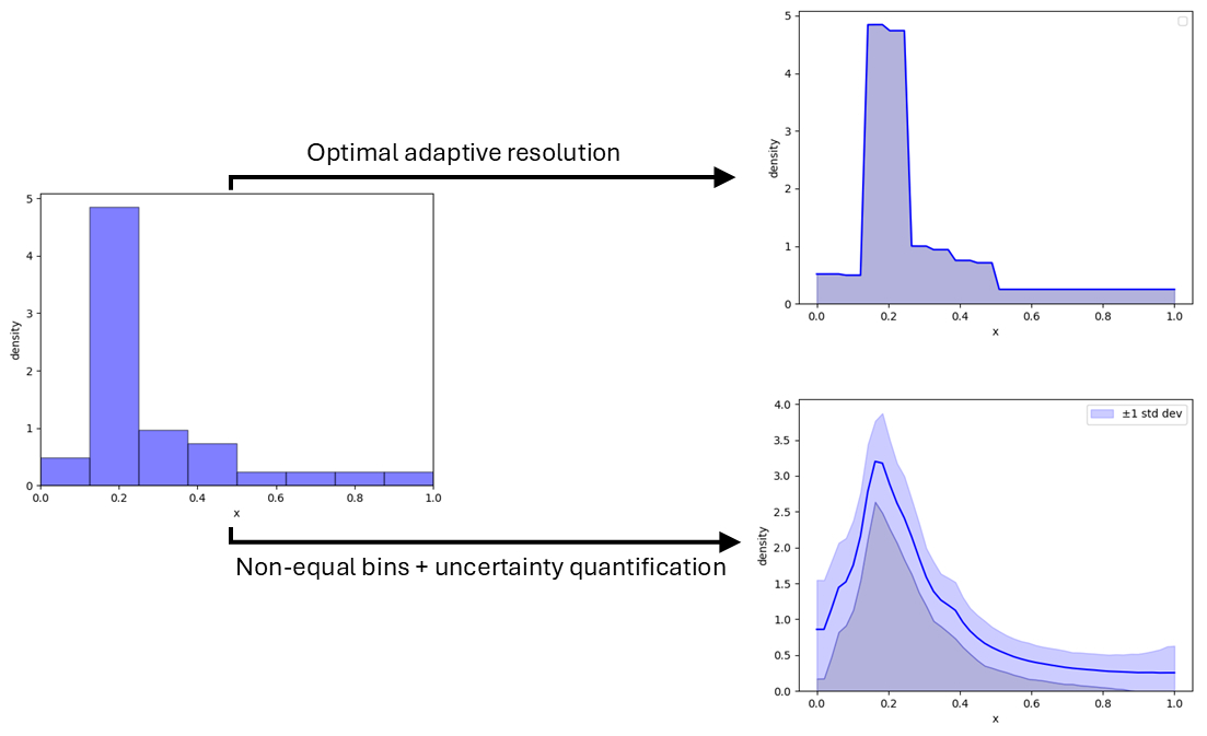
Densities with unequal bins
The beforehand obtained density above appears a bit blocky which originates from the selection of utilizing equal bins. There are different choices accessible akin to taking random splits (and compensating the prior for it). This yields the graph under:

Densities with error bars
Now to shut off the development of densities, it could be of curiosity to visualise our uncertainty in these densities. Though numerically costly to compute, the expression for computing the usual deviation within the density is remarkably simple (F. Pijlman, 2023)
This yields the densities under:


Conclusions
We started with a easy query: Is there a mathematical basis for selecting the bins in a histogram? Because the idea of bins inherently connects knowledge factors with densities, we studied how
to decide on bins for densities.
Utilizing a Bayesian strategy (info idea) one can match densities with out having to fret of overfitting (too many bins exhibiting an excessive amount of element). Though one can compute the “greatest” bin-width, we noticed that:
- Mannequin weighting permits us to mix a number of resolutions, offering a smoother and extra trustworthy illustration of the info.
- Dirichlet Priors give us a rigorous approach to specific our preliminary assumptions about knowledge distribution.
Simply as perturbation idea offers a hierarchy for bodily interactions, this Bayesian framework offers a hierarchy for knowledge decision. The decision scales naturally as extra knowledge turns into accessible. Observe that such concepts can be used when studying fashions by which one has an enlargement in interactions.
The tactic of mixing densities of assorted resolutions was additionally explored in case random bins are chosen. This led to easy histograms which can seem like extra pure for many knowledge
units.
We additionally introduced the usage of normal deviations in histograms. Though the calculation of ordinary deviations was derived for Bayesian fashions, its calculation-procedure suggests a wider applicability. As such, it may be for visualizing the remaining uncertainties in densities.
Acknowledgements
The EdgeAI “Edge AI Applied sciences for Optimised Efficiency Embedded Processing” challenge has acquired funding from Key Digital Applied sciences Joint Enterprise (KDT JU) beneath grant settlement No. 101097300. The KDT JU receives assist from the European Union’s Horizon Europe analysis and innovation program and Austria, Belgium, France, Greece, Italy, Latvia, Luxembourg, Netherlands, and Norway.
References
- F. Pijlman, J. L. (2023). Variance of Probability of Knowledge. https://sitb2023.ulb.be/proceedings/, 34/37.
- Murphy, Okay. (2022). Probabilistic Machine Studying: An Introduction. MIT Press.
- Vries, B. d. (2026). Energetic Inference for Bodily AI Brokers. arXiv.
Bio
Fetze Pijlman is a Principal Scientist at Signify Analysis in Eindhoven, the Netherlands. His analysis focus spans probabilistic machine studying, Bayesian inference, and sign processing, with a selected curiosity in making use of these mathematical frameworks to IoT, sensing, and good methods.


