


# Introduction
Anybody who has spent a good period of time doing information science might in the end study one thing: the golden rule of downstream machine studying modeling, often called rubbish in, rubbish out (GIGO).
For instance, feeding a linear regression mannequin with extremely collinear information, or operating ANOVA assessments on heteroscedastic variances, is the right recipe… for ineffective fashions that will not study correctly.
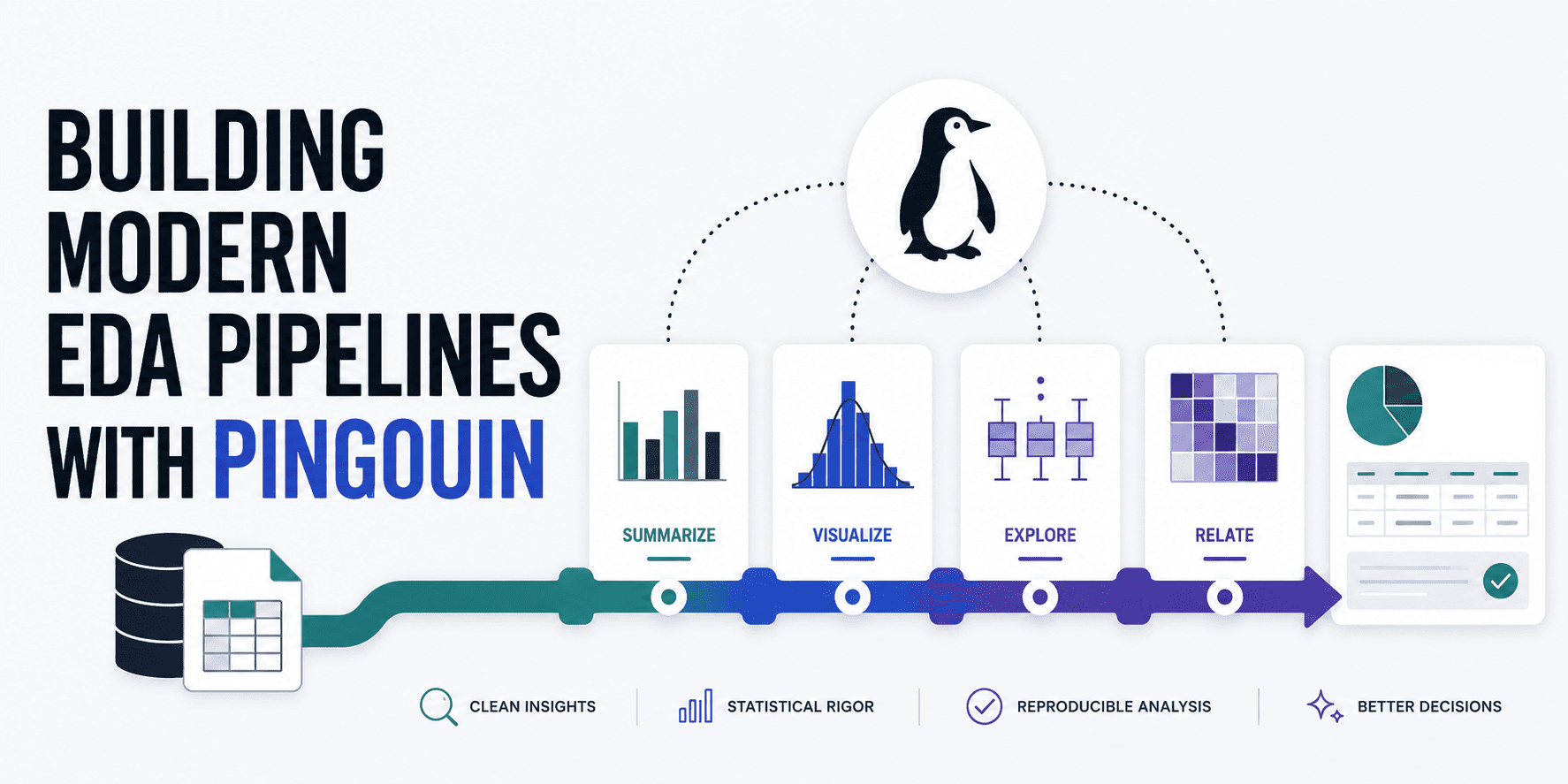
Exploratory information evaluation (EDA) has so much to say when it comes to visualizations like scatter plots and histograms, but they don’t seem to be ample after we want rigorous validation of knowledge in opposition to the mathematical assumptions wanted in downstream analyses or fashions. Pingouin helps do that by bridging the hole between two well-known libraries in information science and statistics: SciPy and pandas. Additional, it may be a fantastic ally to construct strong, automated EDA pipelines. This text teaches you find out how to construct a holistic pipeline for rigorous, statistical EDA, validating a number of essential information properties.
# Preliminary Setup
Let’s begin by ensuring we set up Pingouin in our Python atmosphere (and pandas, in case you do not have it but):
!pip set up pingouin pandas
After that, it is time to import these key libraries and cargo our information. For instance open dataset, we’ll use one containing samples of wine properties and their high quality.
import pandas as pd
import pingouin as pg

# Loading the wine dataset from an open dataset GitHub repository
url = "https://uncooked.githubusercontent.com/gakudo-ai/open-datasets/refs/heads/important/wine-quality-white-and-red.csv"
df = pd.read_csv(url)

# Displaying the primary few rows to know our options
df.head()
# Checking Univariate Normality
The primary of the precise exploratory analyses we’ll conduct pertains to a verify on univariate normality. Many conventional algorithms for coaching machine studying fashions — and statistical assessments like ANOVAs and t-tests, for that matter — want the idea that steady variables observe a traditional, a.ok.a. Gaussian distribution. Pingouin’s pg.normality() perform helps do that verify by a Shapiro-Wilk take a look at throughout the complete dataframe:
# Choosing a subset of steady options for normality checks
options = ['fixed acidity', 'volatile acidity', 'citric acid', 'pH', 'alcohol']

# Working the normality take a look at
normality_results = pg.normality(df[features])
print(normality_results)
Output:
                         W          pval  regular
mounted acidity     0.879789  2.437973e-57   False
unstable acidity  0.875867  6.255995e-58   False
citric acid       0.964977  5.262332e-37   False
pH                0.991448  2.204049e-19   False
alcohol           0.953532  2.918847e-41   False
It looks as if not one of the numeric options at hand fulfill normality. That is on no account one thing incorrect with the info; it is merely a part of its traits. We’re simply getting the message that, in later information preprocessing steps past our EDA, we’d wish to think about making use of information transformations like log-transform or Field-Cox that make the uncooked information look “extra normal-like” and thus extra appropriate for fashions that assume normality.
# Checking Multivariate Normality
Equally, evaluating normality not characteristic by characteristic, however accounting for the interplay between options, is one other attention-grabbing facet to examine. Let’s examine find out how to verify for multivariate normality: a key requirement in strategies like multivariate ANOVA (MANOVA), for example.
# Henze-Zirkler multivariate normality take a look at
multivariate_normality_results = pg.multivariate_normality(df[features])
print(multivariate_normality_results)
Output:
HZResults(hz=np.float64(23.72107048442373), pval=np.float64(0.0), regular=False)
And guess what: chances are you’ll get one thing like HZResults(hz=np.float64(23.72107048442373), pval=np.float64(0.0), regular=False), which suggests multivariate normality does not maintain both. If you’re going to practice a machine studying mannequin on this dataset, this implies non-parametric, tree-based fashions like gradient boosting and random forests may be a extra sturdy different than parametric, weight-based fashions like SVM, linear regression, and so forth.
# Checking Homoscedasticity
Subsequent comes a tough phrase for a somewhat easy idea: homoscedasticity. This refers to equal or fixed variance throughout errors in predictions, and it’s interpreted as a measure of reliability. We are going to take a look at this property (sorry, too exhausting to jot down its title once more!) with Pingouin’s implementation of Levene’s take a look at, as follows:
# Levene's take a look at for equal variances throughout teams
# 'dv' is the goal, dependent variable, 'group' is the explicit variable
homoscedasticity_results = pg.homoscedasticity(information=df, dv='alcohol', group='high quality')
print(homoscedasticity_results)
Consequence:
                W          pval  equal_var
levene  66.338684  2.317649e-80      False
Since we obtained False as soon as once more, now we have a so-called heteroscedasticity downside, which needs to be accounted for in downstream analyses. One doable means may very well be by using sturdy commonplace errors when coaching regression fashions.
# Checking Sphericity
One other statistical property to research is sphericity, which identifies whether or not the variances of variations between doable pairwise combos of circumstances are equal. Testing this property is often fascinating earlier than operating principal element evaluation (PCA) for dimensionality discount, because it helps us perceive whether or not there are correlations between variables. PCA will probably be rendered somewhat ineffective in case there are usually not any:
# Mauchly's sphericity take a look at
sphericity_results = pg.sphericity(df[features])
print(sphericity_results)
Consequence:
SpherResults(spher=False, W=np.float64(0.004437706589942777), chi2=np.float64(35184.26583883276), dof=9, pval=np.float64(0.0))
Appears like now we have chosen a fairly indomitable, arid dataset! However concern not — this text is deliberately designed to concentrate on the EDA course of and enable you to establish loads of information points like these. On the finish of the day, detecting them and understanding what to do about them earlier than downstream, machine studying evaluation is much better than constructing a probably flawed mannequin. On this case, there’s a catch: now we have a p-value of 0.0, which suggests the null speculation of an identification correlation matrix is rejected, i.e. significant correlations exist between the variables. So if we had loads of options and needed to cut back dimensionality, making use of PCA may be a good suggestion.
# Checking Multicollinearity
Final, we’ll verify multicollinearity: a property that signifies whether or not there are extremely correlated predictors. This may turn into, sooner or later, an undesirable property in interpretable fashions like linear regressors. Let’s verify it:
# Calculating a strong correlation matrix with p-values
correlation_matrix = pg.rcorr(df[features], technique='pearson')
print(correlation_matrix)
Output matrix:
                 mounted acidity unstable acidity citric acid     pH alcohol
mounted acidity                -              ***         ***    ***     ***
unstable acidity         0.219                -         ***    ***      **
citric acid              0.324           -0.378           -    ***
pH                      -0.253            0.261       -0.33      -     ***
alcohol                 -0.095           -0.038       -0.01  0.121       -
Whereas pandas’ corr() can be used, Pingouin’s counterpart makes use of asterisks to point the statistical significance degree of every correlation (* for p < 0.05, ** for p < 0.01, and *** for p < 0.001). A correlation might be statistically vital but nonetheless small in magnitude — multicollinearity turns into a priority when absolutely the worth of the correlation is excessive (sometimes above 0.8). In our case, not one of the pairwise correlations are dangerously giant, with all 5 evaluated options offering largely non-overlapping, distinctive info of their very own for additional analyses.
# Wrapping Up
Via a sequence of examples utilized and defined one after the other, now we have seen find out how to unleash the potential of Pingouin, an open-source Python library, to carry out sturdy, fashionable EDA pipelines that enable you to make higher choices in information preprocessing and downstream analyses primarily based on superior statistical assessments or machine studying fashions, serving to you select the correct actions to carry out and the correct fashions to make use of.
Iván Palomares Carrascosa is a frontrunner, author, speaker, and adviser in AI, machine studying, deep studying & LLMs. He trains and guides others in harnessing AI in the actual world.
# Introduction
Anybody who has spent a good period of time doing information science might in the end study one thing: the golden rule of downstream machine studying modeling, often called rubbish in, rubbish out (GIGO).
For instance, feeding a linear regression mannequin with extremely collinear information, or operating ANOVA assessments on heteroscedastic variances, is the right recipe… for ineffective fashions that will not study correctly.
Exploratory information evaluation (EDA) has so much to say when it comes to visualizations like scatter plots and histograms, but they don’t seem to be ample after we want rigorous validation of knowledge in opposition to the mathematical assumptions wanted in downstream analyses or fashions. Pingouin helps do that by bridging the hole between two well-known libraries in information science and statistics: SciPy and pandas. Additional, it may be a fantastic ally to construct strong, automated EDA pipelines. This text teaches you find out how to construct a holistic pipeline for rigorous, statistical EDA, validating a number of essential information properties.
# Preliminary Setup
Let’s begin by ensuring we set up Pingouin in our Python atmosphere (and pandas, in case you do not have it but):
!pip set up pingouin pandas
After that, it is time to import these key libraries and cargo our information. For instance open dataset, we’ll use one containing samples of wine properties and their high quality.
import pandas as pd
import pingouin as pg

# Loading the wine dataset from an open dataset GitHub repository
url = "https://uncooked.githubusercontent.com/gakudo-ai/open-datasets/refs/heads/important/wine-quality-white-and-red.csv"
df = pd.read_csv(url)

# Displaying the primary few rows to know our options
df.head()
# Checking Univariate Normality
The primary of the precise exploratory analyses we’ll conduct pertains to a verify on univariate normality. Many conventional algorithms for coaching machine studying fashions — and statistical assessments like ANOVAs and t-tests, for that matter — want the idea that steady variables observe a traditional, a.ok.a. Gaussian distribution. Pingouin’s pg.normality() perform helps do that verify by a Shapiro-Wilk take a look at throughout the complete dataframe:
# Choosing a subset of steady options for normality checks
options = ['fixed acidity', 'volatile acidity', 'citric acid', 'pH', 'alcohol']

# Working the normality take a look at
normality_results = pg.normality(df[features])
print(normality_results)
Output:
                         W          pval  regular
mounted acidity     0.879789  2.437973e-57   False
unstable acidity  0.875867  6.255995e-58   False
citric acid       0.964977  5.262332e-37   False
pH                0.991448  2.204049e-19   False
alcohol           0.953532  2.918847e-41   False
It looks as if not one of the numeric options at hand fulfill normality. That is on no account one thing incorrect with the info; it is merely a part of its traits. We’re simply getting the message that, in later information preprocessing steps past our EDA, we’d wish to think about making use of information transformations like log-transform or Field-Cox that make the uncooked information look “extra normal-like” and thus extra appropriate for fashions that assume normality.
# Checking Multivariate Normality
Equally, evaluating normality not characteristic by characteristic, however accounting for the interplay between options, is one other attention-grabbing facet to examine. Let’s examine find out how to verify for multivariate normality: a key requirement in strategies like multivariate ANOVA (MANOVA), for example.
# Henze-Zirkler multivariate normality take a look at
multivariate_normality_results = pg.multivariate_normality(df[features])
print(multivariate_normality_results)
Output:
HZResults(hz=np.float64(23.72107048442373), pval=np.float64(0.0), regular=False)
And guess what: chances are you’ll get one thing like HZResults(hz=np.float64(23.72107048442373), pval=np.float64(0.0), regular=False), which suggests multivariate normality does not maintain both. If you’re going to practice a machine studying mannequin on this dataset, this implies non-parametric, tree-based fashions like gradient boosting and random forests may be a extra sturdy different than parametric, weight-based fashions like SVM, linear regression, and so forth.
# Checking Homoscedasticity
Subsequent comes a tough phrase for a somewhat easy idea: homoscedasticity. This refers to equal or fixed variance throughout errors in predictions, and it’s interpreted as a measure of reliability. We are going to take a look at this property (sorry, too exhausting to jot down its title once more!) with Pingouin’s implementation of Levene’s take a look at, as follows:
# Levene's take a look at for equal variances throughout teams
# 'dv' is the goal, dependent variable, 'group' is the explicit variable
homoscedasticity_results = pg.homoscedasticity(information=df, dv='alcohol', group='high quality')
print(homoscedasticity_results)
Consequence:
                W          pval  equal_var
levene  66.338684  2.317649e-80      False
Since we obtained False as soon as once more, now we have a so-called heteroscedasticity downside, which needs to be accounted for in downstream analyses. One doable means may very well be by using sturdy commonplace errors when coaching regression fashions.
# Checking Sphericity
One other statistical property to research is sphericity, which identifies whether or not the variances of variations between doable pairwise combos of circumstances are equal. Testing this property is often fascinating earlier than operating principal element evaluation (PCA) for dimensionality discount, because it helps us perceive whether or not there are correlations between variables. PCA will probably be rendered somewhat ineffective in case there are usually not any:
# Mauchly's sphericity take a look at
sphericity_results = pg.sphericity(df[features])
print(sphericity_results)
Consequence:
SpherResults(spher=False, W=np.float64(0.004437706589942777), chi2=np.float64(35184.26583883276), dof=9, pval=np.float64(0.0))
Appears like now we have chosen a fairly indomitable, arid dataset! However concern not — this text is deliberately designed to concentrate on the EDA course of and enable you to establish loads of information points like these. On the finish of the day, detecting them and understanding what to do about them earlier than downstream, machine studying evaluation is much better than constructing a probably flawed mannequin. On this case, there’s a catch: now we have a p-value of 0.0, which suggests the null speculation of an identification correlation matrix is rejected, i.e. significant correlations exist between the variables. So if we had loads of options and needed to cut back dimensionality, making use of PCA may be a good suggestion.
# Checking Multicollinearity
Final, we’ll verify multicollinearity: a property that signifies whether or not there are extremely correlated predictors. This may turn into, sooner or later, an undesirable property in interpretable fashions like linear regressors. Let’s verify it:
# Calculating a strong correlation matrix with p-values
correlation_matrix = pg.rcorr(df[features], technique='pearson')
print(correlation_matrix)
Output matrix:
                 mounted acidity unstable acidity citric acid     pH alcohol
mounted acidity                -              ***         ***    ***     ***
unstable acidity         0.219                -         ***    ***      **
citric acid              0.324           -0.378           -    ***
pH                      -0.253            0.261       -0.33      -     ***
alcohol                 -0.095           -0.038       -0.01  0.121       -
Whereas pandas’ corr() can be used, Pingouin’s counterpart makes use of asterisks to point the statistical significance degree of every correlation (* for p < 0.05, ** for p < 0.01, and *** for p < 0.001). A correlation might be statistically vital but nonetheless small in magnitude — multicollinearity turns into a priority when absolutely the worth of the correlation is excessive (sometimes above 0.8). In our case, not one of the pairwise correlations are dangerously giant, with all 5 evaluated options offering largely non-overlapping, distinctive info of their very own for additional analyses.
# Wrapping Up
Via a sequence of examples utilized and defined one after the other, now we have seen find out how to unleash the potential of Pingouin, an open-source Python library, to carry out sturdy, fashionable EDA pipelines that enable you to make higher choices in information preprocessing and downstream analyses primarily based on superior statistical assessments or machine studying fashions, serving to you select the correct actions to carry out and the correct fashions to make use of.
Iván Palomares Carrascosa is a frontrunner, author, speaker, and adviser in AI, machine studying, deep studying & LLMs. He trains and guides others in harnessing AI in the actual world.


