


is on the core of AI infrastructure, powering a number of AI options from Retrieval-Augmented Era (RAG) to agentic expertise and long-term reminiscence. In consequence, the demand for indexing massive datasets is rising quickly. For engineering groups, the transition from a small-scale prototype to a full-scale manufacturing resolution is when the required storage and corresponding invoice for vector database infrastructure begin to turn out to be a major ache level. That is when the necessity for optimization arises.
On this article, I discover the principle approaches for vector database storage optimization: Quantization and Matryoshka Illustration Studying (MRL) and analyze how these strategies can be utilized individually or in tandem to cut back infrastructure prices whereas sustaining high-quality retrieval outcomes.
Deep Dive
The Anatomy of Vector Storage Prices
To grasp methods to optimize an index, we first want to have a look at the uncooked numbers. Why do vector databases get so costly within the first place?
The reminiscence footprint of a vector database is pushed by two main components: precision and dimensionality.
- Precision: An embedding vector is often represented as an array of 32-bit floating-point numbers (Float32). This implies every particular person quantity contained in the vector requires 4 bytes of reminiscence.
- Dimensionality: The upper the dimensionality, the extra “house” the mannequin has to encapsulate the semantic particulars of the underlying information. Fashionable embedding fashions usually output vectors with 768 or 1024 dimensions.
Let’s do the mathematics for the standard 1024-dimensional embedding in a manufacturing setting:
- Base Vector Dimension: 1024 dimensions * 4 bytes = 4 KB per vector.
- Excessive Availability: To make sure reliability, manufacturing vector databases make the most of replication (sometimes an element of three). This brings the true reminiscence requirement to 12 KB per listed vector.
Whereas 12 KB sounds trivial, once you transition from a small proof-of-concept to a manufacturing software ingesting hundreds of thousands of paperwork, the infrastructure necessities explode:
- 1 Million Vectors: ~12 GB of RAM
- 100 Million Vectors: ~1.2 TB of RAM
If we assume cloud storage pricing is about $5 USD per GB/month, an index of 100 million vectors will price about $6,000 USD monthly. Crucially, that is only for the uncooked vectors. The precise index information construction (like HNSW) provides substantial reminiscence overhead to retailer the hierarchical graph connections, making the true price even larger.
As a way to optimize storage and due to this fact decrease prices, there are two important strategies:
Quantization
Quantization is the strategy of decreasing the house (RAM or disk) required to retailer the vector by decreasing precision of its underlying numbers. Whereas a normal embedding mannequin outputs high-precision 32-bit floating-point numbers (float32), storing vectors with that precision is dear, particularly for giant indexes. By decreasing the precision, we will drastically cut back storage prices.
There are three main varieties of quantization utilized in vector databases:
Scalar quantization — That is the most typical kind utilized in manufacturing programs. It reduces precision of the vector’s quantity from float32 (4 bytes) to int8 (1 byte), which supplies as much as 4x storage discount whereas having minimal affect on the retrieval high quality. As well as, the decreased precision accelerates distance calculations when evaluating vectors, due to this fact barely decreasing the latency as nicely.
Binary quantization — That is the intense finish of precision discount. It converts float32 numbers right into a single bit (e.g., 1 if the quantity is > 0, and 0 if <= 0). This delivers an enormous 32x discount in storage. Nonetheless, it usually leads to a steep drop in retrieval high quality since such a binary illustration doesn’t present sufficient precision to explain complicated options and mainly blurs them out.
Product quantization — Not like scalar and binary quantization, which function on particular person numbers, product quantization divides the vector into chunks, runs clustering on these chunks to seek out “centroids”, and shops solely the quick ID of the closest centroid. Whereas product quantization can obtain excessive compression, it’s extremely depending on the underlying dataset’s distribution and introduces computational overhead to approximate the distances throughout search.
Word: As a result of product quantization outcomes are extremely dataset-dependent, we are going to focus our empirical experiments on scalar and binary quantization.
Matryoshka Illustration Studying (MRL)
Matryoshka Illustration Studying (MRL) approaches the storage drawback from a totally completely different angle. As an alternative of decreasing the precision of particular person numbers inside the vector, MRL reduces the general dimensionality of the vector itself.
Embedding fashions that help MRL are skilled to front-load essentially the most crucial semantic data into the earliest dimensions of the vector. Very similar to the Russian nesting dolls that the approach is called after, a smaller, extremely succesful illustration is nested inside the bigger one. This distinctive coaching permits engineers to easily truncate (slice off) the tail finish of the vector, drastically decreasing its dimensionality with solely a minimal penalty to retrieval metrics. For instance, a normal 1024-dimensional vector might be cleanly truncated right down to 256, 128, and even 64 dimensions whereas preserving the core semantic which means. In consequence, this method alone can cut back the required storage footprint by as much as 16x (when shifting from 1024 to 64 dimensions), instantly translating to decrease infrastructure payments.
The Experiment
Word: Full, reproducible code for this experiment is obtainable within the GitHub repository.
Each MRL and quantization are highly effective strategies for locating the precise steadiness between retrieval metrics and infrastructure prices to maintain the product options worthwhile whereas offering high-quality outcomes to customers. To grasp the precise trade-offs of those strategies—and to see what occurs once we push the bounds by combining them—we arrange an experiment.
Right here is the structure of our take a look at setting:
- Vector Database: FAISS, particularly using the HNSW (Hierarchical Navigable Small World) index. HNSW is a graph-based Approximate Nearest Neighbour (ANN) algorithm extensively utilized in vector databases. Whereas it considerably accelerates retrieval, it introduces compute and storage overhead to keep up the graph relationships between vectors, making optimization on massive indexes much more crucial.
- Dataset: We utilized the mteb/hotpotQA (cc-by-sa-4.0 license) dataset (obtainable through Hugging Face). It’s a sturdy assortment of query/reply pairs, making it perfect for measuring real-world retrieval metrics.
- Index Dimension: To make sure this experiment stays simply reproducible, the index measurement was restricted to 100,000 paperwork. The unique embedding dimension is 384, which supplies a wonderful baseline to show the trade-offs of various approaches.
- Embedding Mannequin: mixedbread-ai/mxbai-embed-xsmall-v1. It is a extremely environment friendly, compact mannequin with native MRL help, offering a fantastic steadiness between retrieval accuracy and pace.
Storage Optimization Outcomes

To match the approaches mentioned above, we measured the storage footprint throughout completely different dimensionalities and quantization strategies.
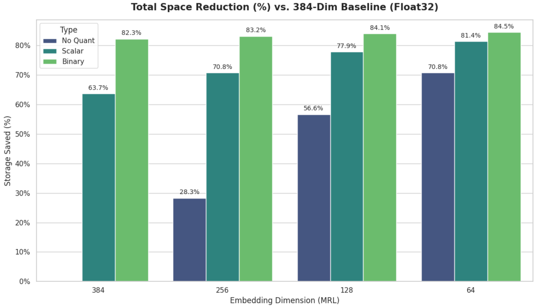
Our baseline for the 100k index (384-dimensional, Float32) began at 172.44 MB. By combining each strategies, the discount is very large:
| Matryoshka dimensionality/quantization strategies | No Quantization (f32) | Scalar (int8) | Binary (1-bit) |
| 384 (Authentic) | 172.44 MB (Ref) | 62.58 MB (63.7% saved) | 30.54 MB (82.3% saved) |
| 256 (MRL) | 123.62 MB (28.3% saved) | 50.38 MB (70.8% saved) | 29.01 MB (83.2% saved) |
| 128 (MRL) | 74.79 MB (56.6% saved) | 38.17 MB (77.9% saved) | 27.49 MB (84.1% saved) |
| 64 (MRL) | 50.37 MB (70.8% saved) | 32.06 MB (81.4% saved) | 26.72 MB (84.5% saved) |
Our information demonstrates that whereas every approach is extremely efficient in isolation, making use of them in tandem yields compounding returns for infrastructure effectivity:
- Quantization: Transferring from Float32 to Scalar (Int8) on the unique 384 dimensions instantly slashes storage by 63.7% (dropping from 172.44 MB to 62.58 MB) with minimal effort.
- MRL: Using MRL to truncate vectors to 128 dimensions—even with none quantization—yields a decent 56.6% discount in storage footprint.
- Mixed Influence: Once we apply Scalar Quantization to a 128-dimensional MRL vector, we obtain an enormous 77.9% discount (bringing the index down to only 38.17 MB). This represents practically a 4.5x enhance in information density with nearly zero architectural modifications to the broader system.
The Accuracy Commerce-off: How a lot can we lose?

Storage optimizations are in the end a trade-off. To grasp the “price” of those optimizations, we evaluated a 100,000-document index utilizing a take a look at set of 1,000 queries from HospotQA dataset. We centered on two main metrics for a retrieval system:
- Recall@10: Measures the system’s skill to incorporate the related doc wherever inside the prime 10 outcomes. That is the crucial metric for RAG pipelines the place an LLM acts as the ultimate arbiter.
- Imply Reciprocal Rank (MRR@10): Measures rating high quality by accounting for the place of the related doc. A better MRR signifies that the “gold” doc is persistently positioned on the very prime of the outcomes.
| Dimension | Kind | Recall@10 | MRR@10 |
| 384 | No Quantization (f32) | 0.481 | 0.367 |
| Scalar (int8) | 0.474 | 0.357 | |
| Binary (1-bit) | 0.391 | 0.291 | |
| 256 | No Quantization (f32) | 0.467 | 0.362 |
| Scalar (int8) | 0.459 | 0.350 | |
| Binary (1-bit) | 0.359 | 0.253 | |
| 128 | No Quantization (f32) | 0.415 | 0.308 |
| Scalar (int8) | 0.410 | 0.303 | |
| Binary (1-bit) | 0.242 | 0.150 | |
| 64 | No Quantization (f32) | 0.296 | 0.199 |
| Scalar (int8) | 0.300 | 0.205 | |
| Binary (1-bit) | 0.102 | 0.054 |
As we will see, the hole between Scalar (int8) and No Quantization is remarkably slim. On the baseline 384 dimensions, the Recall drop is just one.46% (0.481 to 0.474), and the MRR stays practically an identical with only a 2.72% lower (0.367 to 0.357).
In distinction, Binary Quantization (1-bit) represents a “efficiency cliff.” On the baseline 384 dimensions, Binary retrieval already trails Scalar by over 17% in Recall and 18.4% in MRR. As dimensionality drops additional to 64, Binary accuracy collapses to a negligible 0.102 Recall, whereas Scalar maintains a 0.300—making it practically 3x more practical.
Conclusion
Whereas scaling a vector database to billions of vectors is getting simpler, at that scale, infrastructure prices shortly turn out to be a significant bottleneck. On this article, I’ve explored two important strategies for price discount—Quantization and MRL—to quantify potential financial savings and their corresponding trade-offs.
Primarily based on the experiment, there’s little profit to storing information in Float32 so long as high-dimensional vectors are utilized. As we’ve got seen, making use of Scalar Quantization yields an instantaneous 63.7% discount in cupboard space. This considerably lowers total infrastructure prices with a negligible affect on retrieval high quality — experiencing solely a 1.46% drop in Recall@10 and a pair of.72% drop in MRR@10, demonstrating that Scalar Quantization is the best and best infrastructure optimization that the majority RAG use instances ought to undertake.
One other method is combining MRL and Quantization. As proven within the experiment, the mix of 256-dimensional MRL with Scalar Quantization permits us to cut back infrastructure prices even additional by 70.8%. For our preliminary instance of a 100-million, 1024-dimensional vector index, this might cut back prices by as much as $50,000 per yr whereas nonetheless sustaining high-quality retrieval outcomes (experiencing solely a 4.6% discount in Recall@10 and a 4.4% discount in MRR@10 in comparison with the baseline).
Lastly, Binary Quantization: As anticipated, it supplies essentially the most excessive house reductions however suffers from an enormous drop in retrieval metrics. In consequence, it’s way more helpful to use MRL plus Scalar Quantization to attain comparable house discount with a minimal trade-off in accuracy. Primarily based on the experiment, it’s extremely preferable to make the most of decrease dimensionality (128d) with Scalar Quantization—yielding a 77.9% house discount—moderately than utilizing Binary Quantization on the unshortened 384-dimensional index, as the previous demonstrates considerably larger retrieval high quality.
| Technique | Storage Saved | Recall@10 Retention | MRR@10 Retention | Best Use Case |
| 384d + Scalar (int8) | 63.7% | 98.5% | 97.1% | Mission-critical RAG the place the High-1 consequence have to be actual. |
| 256d + Scalar (int8) | 70.8% | 95.4% | 95.6% | The Finest ROI: Optimum steadiness for high-scale manufacturing apps. |
| 128d + Scalar (int8) | 77.9% | 85.2% | 82.5% | Value-sensitive search or 2-stage retrieval (with re-ranking). |
Common Suggestions for Manufacturing Use Instances:
- For a balanced resolution, make the most of MRL + Scalar Quantization. It supplies an enormous discount in RAM/disk house whereas sustaining high-quality retrieval outcomes.
- Binary Quantization needs to be strictly reserved for excessive use instances the place RAM/disk house discount is completely crucial, and the ensuing low retrieval high quality might be compensated for by rising top_k and making use of a cross-encoder re-ranker.
References
[1] Full experiment code https://github.com/otereshin/matryoshka-quantization-analysis
[2] Mannequin https://huggingface.co/mixedbread-ai/mxbai-embed-xsmall-v1
[3] mteb/hotpotqa dataset https://huggingface.co/datasets/mteb/hotpotqa
[4] FAISS https://ai.meta.com/instruments/faiss/
[5] Matryoshka Illustration Studying (MRL): Kusupati, A., Bhatt, G., Rege, A., Wallingford, M., Sinha, A., Ramanujan, V., … & Farhadi, A. (2022). Matryoshka Illustration Studying.


