


Yesterday, we labored with Isolation Forest, which is an Anomaly Detection methodology.
In the present day, we take a look at one other algorithm that has the identical goal. However not like Isolation Forest, it does not construct bushes.
It’s known as LOF, or Native Outlier Issue.
Folks typically summarize LOF with one sentence: Does this level dwell in a area with a decrease density than its neighbors?
This sentence is definitely difficult to grasp. I struggled with it for a very long time.
Nonetheless, there may be one half that’s instantly straightforward to grasp,
and we’ll see that it turns into the important thing level:
there’s a notion of neighbors.
And as quickly as we discuss neighbors,
we naturally return to distance-based fashions.
We’ll clarify this algorithm in 3 steps.
To maintain issues quite simple, we’ll use this dataset, once more:
1, 2, 3, 9
Do you keep in mind that I’ve the copyright on this dataset? We did Isolation Forest with it, and we’ll do LOF with it once more. And we will additionally examine the 2 outcomes.

All of the Excel information can be found by way of this Kofi hyperlink. Your assist means so much to me. The worth will improve throughout the month, so early supporters get the perfect worth.

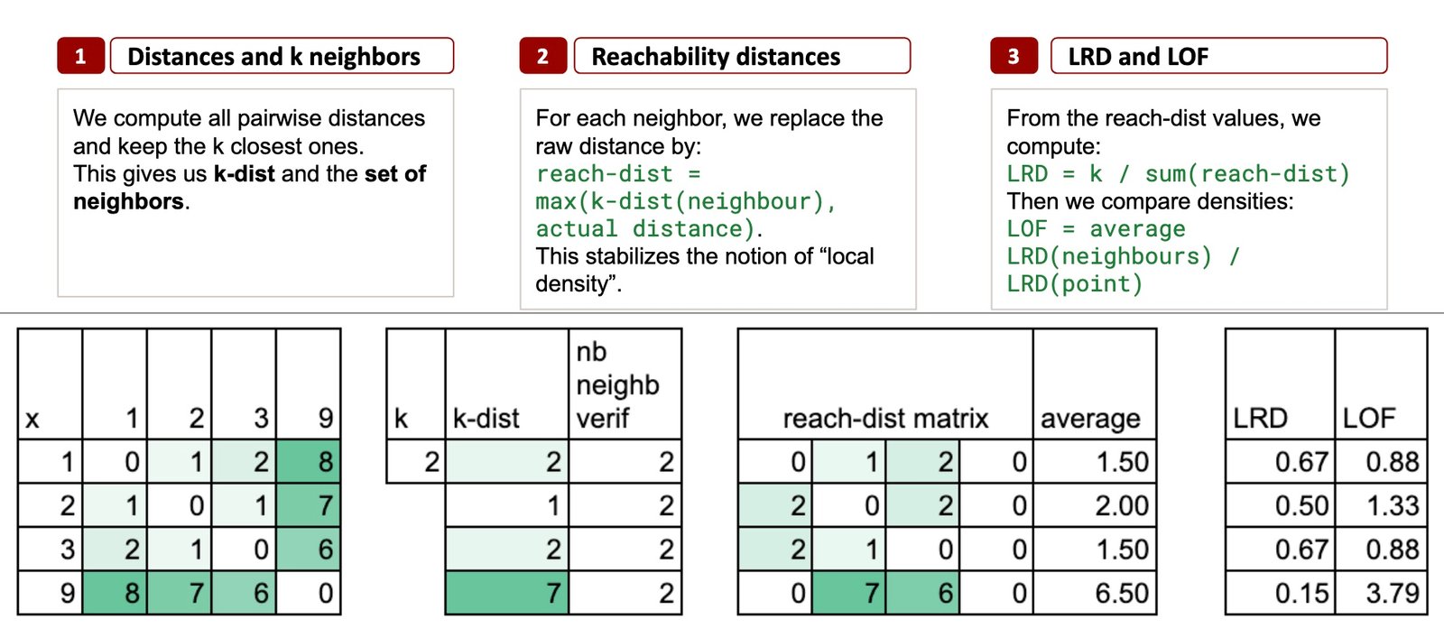
Step 1 – ok Neighbors and k-distance
LOF begins with one thing very simple:
Have a look at the distances between factors.
Then discover the ok nearest neighbors of every level.
Allow us to take ok = 2, simply to maintain issues minimal.
Nearest neighbors for every level
- Level 1 → neighbors: 2 and three
- Level 2 → neighbors: 1 and three
- Level 3 → neighbors: 2 and 1
- Level 9 → neighbors: 3 and a pair of
Already, we see a transparent construction rising:
- 1, 2, and three type a decent cluster
- 9 lives alone, removed from the others
The k-distance: a neighborhood radius
The k-distance is just the biggest distance among the many ok nearest neighbors.
And that is really the important thing level.
As a result of this single quantity tells you one thing very concrete:
the native radius across the level.
If k-distance is small, the purpose is in a dense space.
If k-distance is massive, the purpose is in a sparse space.
With simply this one measure, you have already got a primary sign of “isolation”.
Right here, we use the concept of “ok nearest neighbors”, which in fact reminds us of k-NN (the classifier or regressor).
The context right here is completely different, however the calculation is precisely the identical.
And in case you consider k-means, don’t combine them:
the “ok” in k-means has nothing to do with the “ok” right here.
The k-distance calculation
For level 1, the 2 nearest neighbors are 2 and 3 (distances 1 and a pair of), so k-distance(1) = 2.
For level 2, neighbors are 1 and 3 (each at distance 1), so k-distance(2) = 1.
For level 3, the 2 nearest neighbors are 1 and 2 (distances 2 and 1), so k-distance(3) = 2.
For level 9, neighbors are 3 and 2 (6 and seven), so k-distance(9) = 7. That is large in comparison with all of the others.
In Excel, we will do a pairwise distance matrix to get the k-distance for every level.

Step 2 – Reachability Distances
For this step, I’ll simply outline the calculations right here, and apply the formulation in Excel. As a result of, to be trustworthy, I by no means succeeded find a very intuitive solution to clarify the outcomes.
So, what’s “reachability distance”?
For some extent p and a neighbor o, we outline this reachability distance as:
reach-dist(p, o) = max(k-dist(o), distance(p, o))
Why take the utmost?
The aim of reachability distance is to stabilize density comparability.
If the neighbor o lives in a really dense area (small k-dist), then we don’t wish to permit an unrealistically small distance.
Particularly, for level 2:
- Distance to 1 = 1, however k-distance(1) = 2 → reach-dist(2, 1) = 2
- Distance to three = 1, however k-distance(3) = 2 → reach-dist(2, 3) = 2
Each neighbors drive the reachability distance upward.
In Excel, we’ll preserve a matrix format to show the reachability distances: one level in comparison with all of the others.

Common reachability distance
For every level, we will now compute the common worth, which tells us: on common, how far do I have to journey to succeed in my native neighborhood?
And now, do you discover one thing: the purpose 2 has a bigger common reachability distance than 1 and three.
This isn’t that intuitive to me!
Step 3 – LRD and the LOF Rating
The ultimate step is sort of a “normalization” to seek out an anomaly rating.
First, we outline the LRD, Native Reachability Density, which is just the inverse of the common reachability distance.
And the ultimate LOF rating is calculated as:

So, LOF compares the density of some extent to the density of its neighbors.
Interpretation:
- If LRD(p) ≈ LRD (neighbors), then LOF ≈ 1
- If LRD(p) is way smaller, then LOF >> 1. So p is in a sparse area
- If LRD(p) is way bigger → LOF < 1. So p is in a really dense pocket.
I additionally did a model with extra developments, and shorter formulation.

Understanding What “Anomaly” Means in Unsupervised Fashions
In unsupervised studying, there isn’t any floor fact. And that is precisely the place issues can turn out to be difficult.
We wouldn’t have labels.
We wouldn’t have the “right reply”.
We solely have the construction of the info.
Take this tiny pattern:
1, 2, 3, 7, 8, 12
(I even have the copyright on it.)
If you happen to take a look at it intuitively, which one appears like an anomaly?
Personally, I’d say 12.
Now allow us to take a look at the outcomes. LOF says the outlier is 7.
(And you’ll discover that with k-distance, we’d say that it’s 12.)

Now, we will examine Isolation Forest and LOF aspect by aspect.
On the left, with the dataset 1, 2, 3, 9, each strategies agree:
9 is the clear outlier.
Isolation Forest provides it the bottom rating,
and LOF provides it the very best LOF worth.
If we glance nearer, for Isolation Forest: 1, 2 and three haven’t any variations in rating. And LOF provides the next rating for two. That is what we already seen.
With the dataset 1, 2, 3, 7, 8, 12, the story modifications.
- Isolation Forest factors to 12 as probably the most remoted level.
This matches the instinct: 12 is much from everybody. - LOF, nevertheless, highlights 7 as a substitute.

So who is correct?
It’s tough to say.
In apply, we first have to agree with enterprise groups on what “anomaly” really means within the context of our information.
As a result of in unsupervised studying, there isn’t any single fact.
There may be solely the definition of “anomaly” that every algorithm makes use of.
This is the reason this can be very necessary to grasp
how the algorithm works, and what sort of anomalies it’s designed to detect.
Solely then are you able to resolve whether or not LOF, or k-distance, or Isolation Forest is the best selection on your particular scenario.
And that is the entire message of unsupervised studying:
Totally different algorithms take a look at the info in another way.
There isn’t any “true” outlier.
Solely the definition of what an outlier means for every mannequin.
This is the reason understanding how the algorithm works
is extra necessary than the ultimate rating it produces.
LOF Is Not Actually a Mannequin
There may be another level to make clear about LOF.
LOF doesn’t study a mannequin within the regular sense.
For instance
- k-means learns and retailer centroids (means)
- GMM learns and retailer means and variances
- choice bushes, study and retailer guidelines
All of those produce a operate which you could apply to new information.
And LOF doesn’t produce such a operate. It relies upon fully on the neighborhood construction contained in the dataset. If you happen to add or take away some extent, the neighborhood modifications, the densities change, and the LOF values have to be recalculated.
Even in case you preserve the entire dataset, like k-NN does, you continue to can’t apply LOF safely to new inputs. The definition itself doesn’t generalize.
Conclusion
LOF and Isolation Forest each detect anomalies, however they take a look at the info by way of fully completely different lenses.
- k-distance captures how far some extent should journey to seek out its neighbors.
- LOF compares native densities.
- Isolation Forest isolates factors utilizing random splits.
And even on quite simple datasets, these strategies can disagree.
One algorithm could flag some extent as an outlier, whereas one other highlights a totally completely different one.
And that is the important thing message:
In unsupervised studying, there isn’t any “true” outlier.
Every algorithm defines anomalies in keeping with its personal logic.
This is the reason understanding how a technique works is extra necessary than the quantity it produces.
Solely then are you able to select the best algorithm for the best scenario, and interpret the outcomes with confidence.


