Energy Evaluation in Advertising and marketing: A Palms-On Introduction

Present code

library(tibble)
library(ggplot2)
library(dplyr)
library(tidyr)
library(latex2exp)
library(scales)
library(knitr)

Over the previous few years working in advertising measurement, I’ve observed that energy evaluation is among the most poorly understood testing and measurement matters. Generally it’s misunderstood and typically it’s not utilized in any respect regardless of its foundational function in check design. This text and the sequence that comply with are my makes an attempt to alleviate this.

On this section, I’ll cowl:

Information Visualization Defined (Half 5): Visualizing Time-Sequence Information in Python (Matplotlib, Plotly, and Altair)

Tips on how to Use Gemini 3 Professional Effectively

What’s statistical energy?
How can we compute it?
What can affect energy?

Energy evaluation is a statistical subject and as a consequence, there will probably be math and statistics (loopy proper?) however I’ll attempt to tie these technical particulars again to actual world issues or primary instinct each time potential.

With out additional ado, let’s get to it.

Error sorts in testing: Kind I vs. Kind II

In testing, there are two kinds of error:

Kind I:
- Technical Definition: We erroneously reject the null speculation when the null speculation is true
- Layman’s Definition: We are saying there was an impact when there actually wasn’t
- Instance: A/B testing a brand new inventive and concluding that it performs higher than the previous design when in actuality, each designs carry out the identical
Kind II:
- Technical Definition: We fail to reject the null speculation when the null speculation is fake
- Layman’s Definition: We are saying there was no impact when there actually was
- Instance: A/B testing a brand new inventive and concluding that it performs the identical because the previous design when in actuality, the brand new design performs higher

What’s statistical energy?

Most individuals are aware of Kind I error. It’s the error that we management by setting a significance stage. Energy pertains to Kind II error. Extra particularly, energy is the chance of appropriately rejecting the null speculation when it’s false. It’s the complement of Kind II error (i.e., 1 – Kind II error). In different phrases, energy is the chance of detecting a real impact if one exists. It must be clear why that is vital:

Underpowered assessments are prone to miss true results, resulting in missed alternatives for enchancment
Underpowered assessments can result in false confidence within the outcomes, as we could conclude that there isn’t any impact when there really is one
… and most easily, underpowered assessments waste cash and sources

The function of α and β

If each are vital, why are Kind II error and energy so misunderstood and ignored whereas Kind I is all the time thought-about? It’s as a result of we will simply choose our Kind I error charge. In actual fact, that’s precisely what we’re doing once we set the importance stage α (usually α = 0.05) for our assessments. We’re stating that we’re snug with a sure proportion of Kind I error. Throughout check setup, we make an announcement, “we’re snug with an X % false optimistic charge,” after which set α = X %. After the check, if our p-value falls under α, we reject the null speculation (i.e., “the outcomes are vital”), and if the p-value falls above α, we fail to reject the null speculation (i.e., “the outcomes usually are not vital”).

Figuring out Kind II error, β (usually β = 0.20), and thus energy, isn’t as easy. It requires us to make assumptions and carry out evaluation, known as “energy evaluation.” To know the method, it’s finest to first stroll by the method of testing after which backtrack to determine how energy could be computed and influenced. Let’s use a easy A/B inventive check for instance.

Idea	Image	Typical Worth(s)	Technical Definition	Plain-Language Definition
Kind I Error	α	0.05 (5%)	Chance of rejecting the null speculation when the null is definitely true	Saying there may be an impact when in actuality there isn’t any distinction
Kind II Error	β	0.20 (20%)	Chance of failing to reject the null speculation when the null is definitely false	Saying there isn’t any impact when in actuality there may be one
Energy	1 − β	0.80 (80%)	Chance of appropriately rejecting the null speculation when the choice is true	The possibility we detect a real impact if there may be one

Fast Reference: Error Sorts and Energy

Computing energy: step-by-step

A pair notes earlier than we get began:

I made just a few assumptions and approximations to simplify the instance. In case you can spot them, nice. If not, don’t fear about it. The aim is to know the ideas and course of, not the nitty gritty particulars.
I consult with the choice threshold within the z-score area because the important worth. Vital worth usually refers back to the threshold within the unique area (e.g., conversion charges) however I’ll use it interchangeably so I don’t have to introduce a brand new time period.
There are code snippets all through tied to the textual content and ideas. In case you copy the code your self, you may mess around with the parameters to see how issues change. Among the code snippets are hidden to maintain the article readable. Click on “Present the code” to see the code.
- Do that: Edit the pattern measurement within the check setup in order that the check statistic is just under the important worth after which run the ability evaluation. Are the outcomes what you anticipated?

Check setup and the check statistic

As acknowledged above, it’s finest to stroll by the testing course of first after which backtrack to determine how energy could be computed. Let’s just do that.

# Set parameters for the A/B check
N_a <- 1000  # Pattern measurement for inventive A
N_b <- 1000  # Pattern measurement for inventive B
alpha <- 0.05  # Significance stage
# Perform to compute the important z-value for a one-tailed check
critical_z <- operate(alpha, two_sided = FALSE) {
  if (two_sided) qnorm(1 - alpha/2) else qnorm(1 - alpha)
}

As acknowledged above, it’s finest to stroll by the testing course of first after which backtrack to determine how energy could be computed. Let’s just do that.

Our check setup:

Null speculation: The conversion charge of A equals the conversion charge of B.
Different speculation: The conversion charge of B is bigger than the conversion charge of A.
Pattern measurement:
N_a = 1,000 — Quantity of people that obtain inventive A
N_b = 1,000 — Quantity of people that obtain inventive B
Significance stage: α = 0.05
Vital worth: The important worth is the z-score that corresponds to the importance stage α. We name this Z_1−α. For a one-tailed check with α = 0.05, that is roughly 1.64.
Check sort: Two-proportion z-test

x_a <- 100  # Variety of conversions for inventive A
x_b <- 150  # Variety of conversions for inventive B
p_a <- x_a / N_a  # Conversion charge for inventive A
p_b <- x_b / N_b  # Conversion charge for inventive B

Our outcomes:

x_a = 100 — Variety of conversions from inventive A
x_b = 150 — Variety of conversions from inventive B
p_a = x_a / N_a = 0.10 — Conversion charge of inventive A
p_b = x_b / N_b = 0.15 — Conversion charge of inventive B

Underneath the null speculation, the distinction in conversion charges follows an roughly regular distribution with:

Imply: μ = 0 (no distinction in conversion charges)
Commonplace deviation:
σ = √[ p_a(1 − p_a)/N_a + p_b(1 − p_b)/N_b ] ≈ 0.01

z_score <- operate(p_a, p_b, N_a, N_b) {
  (p_b - p_a) / sqrt((p_a * (1 - p_a) / N_a) + (p_b * (1 - p_b) / N_b))
}

From these values, we will compute the check statistic:

[
z = frac{p_b – p_a}
{sqrt{frac{p_a (1 – p_a)}{N_a} + frac{p_b (1 – p_b)}{N_b}}}
approx 3.39
]

If our check statistic, z, is bigger than the important worth, we reject the null speculation and conclude that Artistic B performs higher than Artistic A. If z is lower than or equal to the important worth, we fail to reject the null speculation and conclude that there isn’t any vital distinction between the 2 creatives.

In different phrases, if our outcomes are unlikely to be noticed when the conversion charges of A and B are really the identical, we reject the null speculation and state that Artistic B performs higher than Artistic A. In any other case, we fail to reject the null speculation and state that there isn’t any vital distinction between the 2 creatives.

Given our check outcomes, we reject the null speculation and conclude that Artistic B performs higher than Artistic A.

z <- z_score(p_a, p_b, N_a, N_b)
critical_value <- critical_z(alpha)
if (z > critical_value) {
  end result <- "Reject null speculation: Artistic B performs higher than Artistic A"
} else {
  end result <- "Fail to reject null speculation: No vital distinction between creatives"
}
end result
#> [1] "Reject null speculation: Artistic B performs higher than Artistic A"

The instinct behind energy

Now that now we have walked by the testing course of, the place does energy come into play? Within the course of above, we file pattern conversion charges, p_a and p_b, after which compute the check statistic, z. Nevertheless, if we repeated the check many occasions, we’d get completely different pattern conversion charges and completely different check statistics, all centering across the true conversion charges of the creatives.

Assume the true conversion charge of Artistic B is greater than that of Artistic A. A few of these assessments will nonetheless fail to reject the null speculation attributable to pure variance. Energy is the share of those assessments that reject the null speculation. That is the underlying mechanism behind all energy evaluation and hints on the lacking ingredient: the true conversion charges—or extra usually, the true impact measurement.

Intuitively, if the true impact measurement is greater, our measured impact would usually be greater and we might reject the null speculation extra usually, rising energy.

Selecting the true impact measurement

If we’d like true conversion charges to compute energy, how can we get them? If we had them, we wouldn’t have to carry out testing. Due to this fact, we have to make an assumption. Broadly, there are two approaches:

Select the significant impact measurement: On this strategy, we assign the true impact measurement (or true distinction in conversion charges) to a stage that will be significant. If Artistic B solely elevated conversion charges by 0.01%, would we really care and take motion on these outcomes? In all probability not. So why would we care about with the ability to detect that small of an impact? Alternatively, if Artistic B elevated conversion charges by 50%, we actually would care. In apply, the significant impact measurement possible falls between these two factors.
- Be aware: That is also known as the minimal detectable impact. Nevertheless, the minimal detectable impact of the research and the minimal detectable impact that we care about (for instance, we could solely care about 5% or better results, however the research is designed to detect 1% or better results) could differ. For that cause, I choose to make use of the time period significant impact when referring to this technique.
Use prior research: If now we have information from prior research or fashions that measure the effectivity of this inventive or comparable creatives, we will use these values to assign the true impact measurement.

Each of the above approaches are legitimate.

In case you solely care to see significant results and don’t thoughts if you happen to miss out on detecting smaller results, go together with the primary choice. In case you should see “statistical significance”, go together with the second choice and be conservative with the values you employ (extra on that in one other article).

Technical Be aware

As a result of we don’t have true conversion charges, we’re technically assigning a selected anticipated distribution to the choice speculation after which computing energy based mostly on that. The true imply within the following passages is technically the anticipated imply below the choice speculation. I’ll use the time period true to maintain the language easy and concise.

Computing and visualizing energy

Now that now we have the lacking elements, true conversion charges, we will compute energy. As a substitute of the measured p_a and p_b, we now have true conversion charges r_a and r_b.

We measure energy as:

[
1 – beta = 1 – P(z < Z_{1-alpha} ;|; N_a, N_b, r_a, r_b)
]

This can be complicated at first look, so let’s break it down.
We’re stating that energy (1 − β) is computed by subtracting the Kind II error charge from one. The Kind II error charge is the chance {that a} check ends in a z-score under our significance threshold, given our pattern measurement and true conversion charges r_a and r_b. How can we compute that final half?

In a two-proportion z-score check, we all know that:

Imply: μ = r_b − r_a
Commonplace deviation: σ = √[ r_a(1 − r_a)/N_a + r_b(1 − r_b)/N_b ]

Now we have to compute:

[
P(X > Z_{1-alpha}), quad X sim N!left(frac{mu}{sigma},,1right)
]

That is the world below the above distribution that lies to the proper of Z_1−α and is equal to computing:

[
P!left(X > frac{mu}{sigma} – Z_{1-alpha}right), quad X sim N(0,1)
]

If we had a textbook with a z-score desk, we might merely search for the p-value related to
(μ / σ − Z_1−α), and that will give us the ability.

Let’s present this visually:

Present the code

r_a <- p_a  # true baseline conversion charge; we're reusing the measured worth
r_b <- p_b   # true remedy conversion charge; we're reusing the measure worth
alpha <- 0.05
two_sided <- FALSE   # set TRUE for two-sided check

mu_diff <- operate(r_a, r_b) r_b - r_a
sigma_diff <- operate(r_a, r_b, N_a, N_b) {
  sqrt(r_a*(1 - r_a)/N_a + r_b*(1 - r_b)/N_b)
}

power_value <- operate(r_a, r_b, N_a, N_b, alpha, two_sided = FALSE) {
  mu <- mu_diff(r_a, r_b)
  sd1 <- sigma_diff(r_a, r_b, N_a, N_b)
  zc <- critical_z(alpha, two_sided)
  thr <- zc * sigma_diff(r_a, r_b, N_a, N_b)  

  if (!two_sided) {
    1 - pnorm(thr, imply = mu, sd = sd1)
  } else {
    pnorm(-thr, imply = mu, sd = sd1) + (1 - pnorm(thr, imply = mu, sd = sd1))
  }
}

# Construct plot information
mu <- mu_diff(r_a, r_b)
sd1 <- sigma_diff(r_a, r_b, N_a, N_b)
zc <- critical_z(alpha, two_sided)
thr <- zc * sigma_diff(r_a, r_b, N_a, N_b)  

# x-range masking each curves and thresholds
x_min <- min(-4*sd1, mu - 4*sd1, -thr) - 0.1*sd1
x_max <- max( 4*sd1, mu + 4*sd1,  thr) + 0.1*sd1
xx <- seq(x_min, x_max, size.out = 2000)

df <- tibble(
  x = xx,
  H0 = dnorm(xx, imply = 0,  sd = sd1),   # distribution utilized by check threshold
  H1 = dnorm(xx, imply = mu, sd = sd1)    # true (different) distribution
)

# Areas to shade for energy
if (!two_sided) {
  shade <- df %>% filter(x >= thr)
} else {
  shade <- bind_rows(
    df %>% filter(x >=  thr),
    df %>% filter(x <= -thr)
  )
}

# Numeric energy for subtitle
pow <- power_value(r_a, r_b, N_a, N_b, alpha, two_sided)

# Plot
ggplot(df, aes(x = x)) +
  # H1 shaded energy area
  geom_area(
    information = shade, aes(y = H1), alpha = 0.25
  ) +
  # Curves
  geom_line(aes(y = H0), linewidth = 1) +
  geom_line(aes(y = H1), linewidth = 1, linetype = "dashed") +
  # Vital line(s)
  geom_vline(xintercept = thr,  linetype = "dotted", linewidth = 0.8) +
  { if (two_sided) geom_vline(xintercept = -thr, linetype = "dotted", linewidth = 0.8) } +
  # Imply markers
  geom_vline(xintercept = 0,  alpha = 0.3) +
  geom_vline(xintercept = mu, alpha = 0.3, linetype = "dashed") +
  # Labels
  labs(
    title = "Energy as shaded space below H1 past  important threshold",
    subtitle = TeX(sprintf(r"($1 - beta$ = %.1f%%  |  $mu$ = %.4f,  $sigma$ = %.4f,  $z^*$ = %.3f,  threshold = %.4f)",
                       100*pow, mu, sd1, zc, thr)),
    x = TeX(r"(Distinction in conversion charges ($D = p_b - p_a$))"),
    y = "Density"
  ) +
  annotate("textual content", x = mu, y = max(df$H1)*0.95, label = TeX(r"(H1: $N(mu, sigma^2)$)"), hjust = -0.05) +
  annotate("textual content", x = 0,  y = max(df$H0)*0.95, label = TeX(r"(H0: $N(0, sigma^2)$)"),  hjust = 1.05) +
  theme_minimal(base_size = 13)

Within the plot above, energy is the world below the choice distribution (H1) (the place we assume the choice is distributed in keeping with our true conversion charges) that’s past the important threshold (i.e., the world the place we reject the null speculation). With the parameters we set, the ability is 0.96. Because of this if we repeated this check many occasions with the identical parameters, we’d anticipate to reject the null speculation roughly 96% of the time.

Energy curves

Now that now we have instinct and math behind energy, we will discover how energy modifications based mostly on completely different parameters. The plots generated from such evaluation are known as energy curves.

Be aware

All through the plots, you’ll discover that 80% energy is highlighted. This can be a frequent goal for energy in testing, because it balances the chance of Kind II error with the price of rising pattern measurement or adjusting different parameters. You’ll see this worth highlighted in lots of software program packages as a consequence.

Relationship with impact measurement

Earlier, I acknowledged that the bigger the impact measurement, the upper the ability. Intuitively, this is sensible. We’re basically shifting the proper bell curve within the plot above additional to the proper, so the world past the important threshold will increase. Let’s check that concept.

Present the code

# Perform to compute energy for various impact sizes
power_curve <- operate(effect_sizes, N_a, N_b, alpha, two_sided = FALSE) {
  sapply(effect_sizes, operate(e) {
    r_a <- p_a
    r_b <- p_a + e  # Regulate r_b based mostly on impact measurement
    power_value(r_a, r_b, N_a, N_b, alpha, two_sided)
  })
}
# Generate impact sizes
effect_sizes <- seq(0, 0.1, size.out = 100)  # Impact sizes from 0 to 10%
# Compute energy for every impact measurement
power_values <- power_curve(effect_sizes, N_a, N_b, alpha)
# Create an information body for plotting
power_df <- tibble(
  effect_size = effect_sizes,
  energy = power_values
)
# Plot the ability curve
ggplot(power_df, aes(x = effect_size, y = energy)) +
  geom_line(coloration = "blue", measurement = 1) +
  geom_hline(yintercept = 0.80, linetype = "dashed", alpha = 0.6) +  # goal energy information
  labs(
    title = "Energy vs. Impact Measurement",
    x = TeX(r"(Impact Measurement ($r_b - r_a$))"),
    y = TeX(r'(Energy ($1 - beta $))')
  ) +
  scale_x_continuous(labels = scales::percent_format(accuracy = 0.01)) +
  scale_y_continuous(labels = scales::percent_format(accuracy = 1), limits = c(NA,1)) +
  theme_minimal(base_size = 13)

Principle confirmed: because the impact measurement will increase, energy will increase. It approaches 100% because the impact measurement will increase and our determination threshold strikes down the long-tail of the traditional distribution.

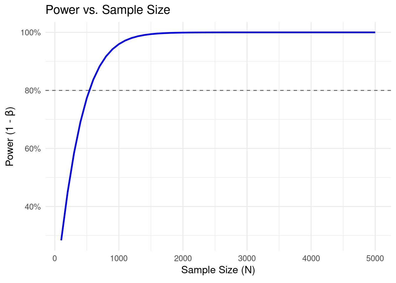
Relationship with pattern measurement

Sadly, we can not management impact measurement. It’s both the significant impact measurement you want to detect or based mostly on prior research. It’s what it’s. What we will management is pattern measurement. The bigger the pattern measurement, the smaller the usual deviation of the distribution and the bigger the world below the curve past the important threshold (think about squeezing the edges to compress the bell curves within the plot earlier). In different phrases, bigger pattern sizes ought to result in greater energy. Let’s check this concept as nicely.

Present the code

power_sample_size <- operate(N_a, N_b, r_a, r_b, alpha, two_sided = FALSE) {
  power_value(r_a, r_b, N_a, N_b, alpha, two_sided)
}
# Generate pattern sizes
sample_sizes <- seq(100, 5000, by = 100)  # Pattern sizes from 100 to 5000
# Compute energy for every pattern measurement
power_values_sample <- sapply(sample_sizes, operate(N) {
  power_sample_size(N, N, r_a, r_b, alpha)
})
# Create an information body for plotting
power_sample_df <- tibble(
  sample_size = sample_sizes,
  energy = power_values_sample
)
# Plot the ability curve for various pattern sizes
ggplot(power_sample_df, aes(x = sample_size, y = energy)) +
  geom_line(coloration = "blue", measurement = 1) +
  geom_hline(yintercept = 0.80, linetype = "dashed", alpha = 0.6) +  # goal energy information
  labs(
    title = "Energy vs. Pattern Measurement",
    x = TeX(r"(Pattern Measurement ($N$))"),
    y = TeX(r"(Energy (1 - $beta$))")
  ) +
  scale_y_continuous(labels = scales::percent_format(accuracy = 1), limits = c(NA,1)) +
  theme_minimal(base_size = 13)

We once more see the anticipated relationship: as pattern measurement will increase, energy will increase.

Be aware

On this particular setup, we will improve energy by rising pattern measurement. Extra usually, this is a rise in precision. In different check setups, precision—and thus energy—could be elevated by different means. For instance, in Geo-testing, we will improve precision by deciding on predictable markets or by the inclusion of exogenous options (extra on this in a future article).

Relationship with significance stage

Does the importance stage α affect energy? Intuitively, if we’re extra keen to just accept Kind I error, we usually tend to reject the null speculation and thus (1 − β) must be greater. Let’s check this concept.

Present the code

power_of_alpha <- operate(alpha_vec, r_a, r_b, N_a, N_b, two_sided = FALSE) {
  sapply(alpha_vec, operate(a)
    power_value(r_a, r_b, N_a, N_b, a, two_sided)
  )
}

alpha_grid <- seq(0.001, 0.20, size.out = 400)
power_grid <- power_of_alpha(alpha_grid, r_a, r_b, N_a, N_b, two_sided)

# Present level
power_now <- power_value(r_a, r_b, N_a, N_b, alpha, two_sided)

df_alpha_power <- tibble(alpha = alpha_grid, energy = power_grid)

ggplot(df_alpha_power, aes(x = alpha, y = energy)) +
  geom_line(coloration = "blue", measurement = 1) +
  geom_hline(yintercept = 0.80, linetype = "dashed", alpha = 0.6) +  # goal energy information
  geom_vline(xintercept = alpha, linetype = "dashed", alpha = 0.6) + # your alpha
  scale_x_continuous(labels = scales::percent_format(accuracy = 1)) +
  scale_y_continuous(labels = scales::percent_format(accuracy = 1), limits = c(NA,1)) +
  labs(
    title = TeX(r"(Energy vs. Significance Degree)"),
    subtitle = TeX(sprintf(r"(At $alpha$ = %.1f%%, $1 - beta$ = %.1f%%)",
                       100*alpha, 100*power_now)),
    x = TeX(r"(Significance Degree ($alpha$))"),
    y = TeX(r"(Energy (1 - $beta$))")
  ) +
  theme_minimal(base_size = 13)

But once more, the outcomes match our instinct. There is no such thing as a free lunch in statistics. All else equal, if we need to lower our Kind II error charge (β), we should be keen to just accept the next Kind I charge (α).

Energy evaluation

So what’s energy evaluation? Energy evaluation is the method of computing energy given the parameters of the check. In energy evaluation, we repair parameters we can not management after which optimize the parameters we will management to realize a desired energy stage. For instance, we will repair the true impact measurement after which compute the pattern measurement wanted to realize a desired energy stage. Energy curves are sometimes used to help with this decision-making course of. Later within the sequence, I’ll stroll by energy evaluation intimately with a real-world instance.