


To get probably the most out of this tutorial, you must have a stable understanding of the way to examine two distributions. In case you don’t, I like to recommend testing this wonderful article by @matteo-courthoud.
We automated the evaluation and exported the outcomes to an Excel file utilizing Python. In case you already know the fundamentals of Python and the way to write to Excel, that may make issues even simpler.
I wish to thank everybody who took the time to learn and interact with my article. Your help and suggestions imply loads.
, whether or not tutorial or skilled, the query of knowledge representativeness between two samples arises steadily.
By representativeness, we imply the diploma to which two samples resemble one another or share the identical traits. This idea is important, because it immediately determines the accuracy of statistical conclusions or the efficiency of a predictive mannequin.
At every stage of a mannequin’s life cycle, the difficulty of knowledge representativeness takes particular kinds :
- Throughout the development section: that is the place all of it begins. You collect the information, clear it, cut up it into coaching, check, and out-of-time samples, estimate the parameters, and punctiliously doc each determination. You make sure that the check and the out-of-time samples are consultant of the coaching information.
- In The applying section: as soon as the mannequin is constructed, it should be confronted with actuality. And right here an important query arises: do the brand new datasets actually resemble those used throughout building? If not, a lot of the earlier work could shortly lose its worth.
- In the monitoring section, or backtesting: over time, populations evolve. The mannequin should due to this fact be repeatedly challenged. Do its predictions stay legitimate? Is the representativeness of the goal portfolio nonetheless ensured?
Representativeness is due to this fact not a one-off constraint, however a problem that accompanies the mannequin all through its improvement.
To reply the query of representativeness between two samples, the commonest method is to match their distributions, proportions, and buildings. This includes the usage of visible instruments like density features, histograms, boxplots, supplemented by statistical exams such because the Scholar’s t-test, the Kruskal-Wallis check, the Wilcoxon check, or the Kolmogorov-Smirnov check. On this topic, @matteo-courthoud has printed an important article, full with sensible codes, to which we refer the reader for additional info.
On this article, we’ll concentrate on two sensible instruments usually utilized in credit score danger administration to examine whether or not two datasets are comparable:
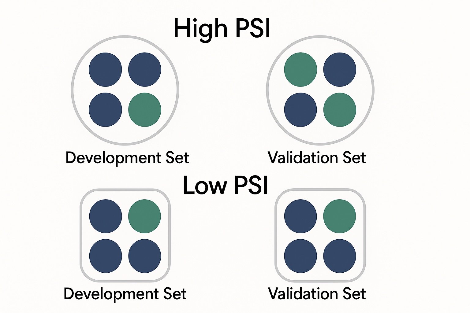
- The Inhabitants Stability Index (PSI) exhibits how a lot a distribution shifts, both over time or between two samples.
- Cramér’s V measures the energy of affiliation between classes, serving to us see if two populations share an analogous construction.
We are going to then discover how these instruments may also help engineers and decision-makers by reworking statistical comparisons into clear information for sooner and extra dependable selections.
In Part 1 of this text, we current two concrete examples the place questions of representativeness between samples could come up. In Part 2, we consider representativeness between two datasets utilizing PSI and Cramér’s V. Lastly, in Part 3, we display the way to implement and automate these analyses in Python, exporting the outcomes into an Excel file.
1. Two real-world examples of the representativeness problem
The difficulty of representativeness turns into necessary when a mannequin is utilized to a website apart from the one for which it was developed. Two typical conditions illustrate this problem:
1.1 When a mannequin is utilized to a new scope of purchasers
Think about a financial institution growing a scoring mannequin for small companies. The mannequin performs effectively and is acknowledged internally. Inspired by this success, the management decides to increase its use to massive companies. Your supervisor asks in your opinion on the method. What steps do you’re taking earlier than responding?
Because the improvement and software populations differ, utilizing the mannequin on the brand new inhabitants extends its scope. It’s due to this fact essential to verify that this software is legitimate.
The statistician has a number of instruments to handle this query, specifically representativeness evaluation evaluating the event inhabitants with the appliance inhabitants. This may be achieved by analyzing their traits variable by variable, for instance by means of exams of imply equality, exams of distribution equality, or by evaluating the distribution of categorical variables.
1.2 When two banks merge and must align their danger fashions
Now think about Financial institution A, a big establishment with a considerable stability sheet and a confirmed mannequin to evaluate shopper default danger. Financial institution A is finding out the potential for merging with Financial institution B. Financial institution B, nonetheless, operates in a weaker financial surroundings and has not developed its personal inside mannequin.
Suppose Financial institution A’s administration approaches you, because the statistician liable for its inside fashions. The strategic query is: wouldn’t it be acceptable to use Financial institution A’s inside fashions to Financial institution B’s portfolio within the occasion of a merger?
Earlier than making use of Financial institution A’s inside mannequin to Financial institution B’s portfolio, it’s essential to match the distributions of key variables throughout each portfolios. The mannequin can solely be transferred with confidence if the 2 populations are actually consultant of one another.
We’ve simply introduced two concrete instances the place verifying representativeness is important for sound decision-making. Within the subsequent part, we deal with the way to analyze representativeness between two portfolios by introducing two statistical instruments: the Inhabitants Stability Index (PSI) and Cramér’s V.
2. Evaluating Distributions to Assess Representativeness Between Two Populations Utilizing the Inhabitants Stability Index (PSI) and V-Cramer.
In observe, the examine of representativeness between two datasets consists of evaluating the traits of the noticed variables in each samples. This comparability depends on each statistical measures and visible instruments.
From a statistical perspective, analysts usually look at measures of central tendency (imply, median) and dispersion (variance, customary deviation), in addition to extra granular indicators comparable to quantiles.
On the visible aspect, widespread instruments embody histograms, boxplots, cumulative distribution features, density curves, and QQ-plots. These visualizations assist detect potential variations in form, location, or dispersion between two distributions.
Such graphical analyses present a vital first step: they information the investigation and assist formulate hypotheses. Nevertheless, they should be complemented by statistical exams to verify observations and attain rigorous conclusions. These exams embody:
- Parametric exams, comparable to Scholar’s t-test (comparability of means),
- Nonparametric exams, such because the Kolmogorov–Smirnov check (comparability of distributions), the chi-squared check (for categorical variables), and Welch’s check (for unequal variances).
These approaches are effectively introduced within the article by @matteo-courthoud. Past them, two indicators are notably related in credit score danger evaluation for assessing distributional drift between populations and supporting decision-making: the Inhabitants Stability Index (PSI) and Cramér’s V
2.1. The Inhabitants Stability Index (PSI)
The PSI is a elementary device within the credit score business. It measures the distinction between two distributions of the identical variable:
- for instance, between the coaching dataset and a more moderen software dataset,
- or between a reference dataset at time T0 and one other at time T1.
In different phrases, the PSI quantifies how a lot a inhabitants has drifted over time or throughout completely different scopes.
Right here’s the way it works in observe:
- For a categorical variable, we compute the proportion of observations in every class for each datasets.
- For a steady variable, we first discretize it into bins. In observe, deciles are sometimes used to acquire a balanced distribution.
The PSI then compares, bin by bin, the proportions noticed within the reference dataset versus the goal dataset. The ultimate indicator aggregates these variations utilizing a logarithmic formulation:

Right here, pᵢ and qᵢ symbolize the proportions in bin i for the reference dataset and the goal dataset, respectively. The PSI might be computed simply in an Excel file:

The interpretation is extremely intuitive:
- A smaller PSI means the 2 distributions are nearer.
- A PSI of 0 means the distributions are similar.
- A really massive PSI (tending towards infinity) means the 2 distributions are basically completely different.
In observe, business pointers usually use the next thresholds:
- PSI < 0.1: the inhabitants is secure,
- 0.1 ≤ PSI < 0.25: the shift is noticeable—monitor intently,
- PSI ≥ 0.25: the shift is critical—the mannequin could now not be dependable.
2.2. Cramér’s V
When assessing the representativeness of a categorical variable (or a discretized steady variable) between two datasets, a pure place to begin is the Chi-square check of independence.
We construct a contingency desk crossing:
- the classes (modalities) of the variable of curiosity, and
- an indicator variable for dataset membership (Dataset 1 / Dataset 2).
The check relies on the next statistic:

the place Oij are the noticed counts and Eij are the anticipated counts underneath the idea of independence.
- Null speculation H0: the variable has the identical distribution in each datasets (independence).
- Different speculation H1 : the distributions differ.
If H0 is rejected, we conclude that the variable doesn’t comply with the identical distribution throughout the 2 datasets.
Nevertheless, the Chi-square check has a significant limitation: it solely gives a binary reply (reject / don’t reject), and its energy is extremely delicate to pattern dimension. With very massive datasets, even tiny variations can seem statistically important.
To deal with this limitation, we use Cramér’s V, which rescales the Chi-square statistic to supply a normalized measure of affiliation bounded between 0 and 1:

the place n is the overall pattern dimension, r is the variety of rows, and c is the variety of columns within the contingency desk.
The interpretation is intuitive:
- V≈0 ⇒ The distributions are very related; representativeness is robust.
- V→1 ⇒ The distinction between distributions is massive; the datasets are structurally completely different.
In contrast to the Chi-square check, which merely solutions “sure” or “no,” Cramér’s V gives a graded measure of the energy of the distinction. This permits us to evaluate whether or not the distinction is negligible, average, or substantial.
We use the identical thresholds as these utilized for the PSI to attract our conclusions. For the PSI and Cramér’s V indicators, if the distribution of a number of variables differs considerably between the 2 datasets, we conclude that they aren’t consultant.
3. Measuring Representativeness with PSI and Cramér’s V in Python.
In a earlier article, we utilized completely different variable choice strategies to scale back the Communities & Crime dataset to simply 16 explanatory variables. This step was important to simplify the mannequin whereas protecting probably the most related info.
This dataset additionally features a variable referred to as fold, which splits the information into 10 subsamples. These folds are generally utilized in cross-validation: they permit us to check the robustness of a mannequin by coaching it on one a part of the information and validating it on one other. For cross-validation to be dependable, every fold ought to be consultant of the worldwide dataset:
- To make sure legitimate efficiency estimates.
- To stop bias: a non-representative fold can distort mannequin outcomes
- To help generalization: consultant folds present a greater indication of how the mannequin will carry out on new information.
On this instance, we’ll concentrate on checking whether or not fold 1 is consultant of the worldwide dataset utilizing our two indicators: PSI and Cramer’s V by evaluating the distribution of 16 variables throughout the 2 samples. We are going to proceed in two steps:
Step 1: Begin with the Goal Variable
We start with the goal variable. The concept is straightforward: examine its distribution between fold 1 and your entire dataset. To quantify this distinction, we’ll use two complementary indicators:
- the Inhabitants Stability Index (PSI), which measures distributional shifts,
- Cramér’s V, which measures the energy of affiliation between two categorical variables.
Step 2: Automating the Evaluation for All Variables
After illustrating the method with the goal, we lengthen it to all options. We’ll construct a Python operate that computes PSI and Cramér’s V for every of the 16 explanatory variables, in addition to for the goal variable.
To make the outcomes simple to interpret, we’ll export every little thing into an Excel file with:
- one sheet per variable, displaying the detailed comparability by phase,
- a Abstract tab, aggregating outcomes throughout all variables.
3.1 Evaluating the goal variable ViolentCrimesPerPop between the worldwide dataset (reference) and fold 1 (goal)
Earlier than making use of statistical exams or constructing determination indicators, it’s important to conduct a descriptive and graphical evaluation. There should not simply formalities; they supply an early instinct concerning the variations between populations and assist deciphering the outcomes. In observe, a well-chosen chart usually reveals the conclusions that indicators like PSI or Cramér’s V will later verify (or problem).
For visualization, we proceed in three steps:
1. Evaluating steady distributions We start with graphical instruments comparable to boxplots, cumulative distribution features, and chance density plots. These visualizations present an intuitive technique to look at variations within the goal variable’s distribution between the 2 datasets.
2. Discretization into quantiles Subsequent, we discretize the variable within the reference dataset utilizing quartiles (Q1, Q2, Q3, This autumn), which creates 5 lessons (Q1 by means of Q5). We then apply the very same cut-off factors to the goal dataset, guaranteeing that every statement is mapped to intervals outlined from the reference. This ensures comparability between the 2 distributions.
3. Evaluating categorical distributions Lastly, as soon as the variable has been discretized, we are able to use visualization strategies fitted to categorical information — comparable to bar charts — to match how frequencies are distributed throughout the 2 datasets.
The method relies on the kind of variable:
For a steady variable:
- Begin with customary visualizations (boxplots, cumulative distributions, and density plots).
- Subsequent, cut up the variable into segments (Q1 to Q5) based mostly on the reference dataset’s quantiles.
- Lastly, deal with these segments as classes and examine their distributions.
For a categorical variable:
- No discretization is required — it’s already in categorical kind.
- Go straight to evaluating class distributions, for instance with a bar chart.
The code under prepares the 2 datasets we need to examine after which visualizes the goal variable with a boxplot, displaying its distribution in each the worldwide dataset and in fold 1.
import pandas as pd
import numpy as np
import seaborn as sns
import matplotlib.pyplot as plt
from scipy.stats import chi2_contingency, ks_2samp

information = pd.read_csv("communities_data.csv")
# filter sur fold =1

data_ref = information
data_target = information[data["fold"] == 1]

# examine the 2 distribution of "ViolentCrimesPerPop" within the reference and goal datasets with boxplots


# Construct datasets with a "Group" column
df_ref = pd.DataFrame({
    "ViolentCrimesPerPop": data_ref["ViolentCrimesPerPop"],
    "Group": "Reference"
})

df_target = pd.DataFrame({
    "ViolentCrimesPerPop": data_target["ViolentCrimesPerPop"],
    "Group": "Goal"
})

# Merge them
df_all = pd.concat([df_ref, df_target])


plt.determine(figsize=(8, 6))

# Boxplot with each distributions overlayed
sns.boxplot(
    x="Group",
    y="ViolentCrimesPerPop",
    information=df_all,
    palette="Set2",
    width=0.6,
    fliersize=3
)


# Add imply factors
means = df_all.groupby("Group")["ViolentCrimesPerPop"].imply()
for i, m in enumerate(means):
    plt.scatter(i, m, colour="purple", marker="D", s=50, zorder=3, label="Imply" if i == 0 else "")

# Title tells the story
plt.title("Violent Crimes Per Inhabitants by Group", fontsize=14, weight="daring")
plt.suptitle("Each teams present practically similar distributions",
             fontsize=10, colour="grey")

plt.ylabel("Violent Crimes (Per Pop)", fontsize=12)
plt.xlabel("")

# Cleaner look
sns.despine()
plt.grid(axis="y", linestyle="--", alpha=0.5, seen=False)
plt.legend()

plt.present()


print(len(information.columns))
The determine above means that each teams share related distributions for the ViolentCrimesPerPop variable. To take a more in-depth look, we are able to use Kernel Density Estimation (KDE) plots, which offer a clean view of the underlying distribution and make it simpler to identify delicate variations.
plt.determine(figsize=(8, 6))

# KDE plots with higher styling
sns.kdeplot(
    information=df_all,
    x="ViolentCrimesPerPop",
    hue="Group",
    fill=True,         # use shading for overlap
    alpha=0.4,         # transparency to indicate overlap
    common_norm=False,
    palette="Set2",
    linewidth=2
)

# KS-test for distribution distinction
g1 = df_all[df_all["Group"] == df_all["Group"].distinctive()[0]]["ViolentCrimesPerPop"]
g2 = df_all[df_all["Group"] == df_all["Group"].distinctive()[1]]["ViolentCrimesPerPop"]
stat, pval = ks_2samp(g1, g2)

# Add annotation
plt.textual content(df_all["ViolentCrimesPerPop"].imply(),
         plt.ylim()[1]*0.9,
         f"KS-test p-value = {pval:.3f}nNo important distinction noticed",
         ha="middle", fontsize=10, colour="black")

# Titles with story
plt.title("Kernel Density Estimation of Violent Crimes Per Inhabitants", fontsize=14, weight="daring")
plt.suptitle("Distributions overlap nearly fully between teams", fontsize=10, colour="grey")

plt.xlabel("Violent Crimes (Per Pop)")
plt.ylabel("Density")

sns.despine()
plt.grid(False)
plt.present()
The KDE graph confirms that the 2 distributions are very related, displaying a excessive diploma of overlap. The Kolmogorov-Smirnov (KS) statistical check of 0.976 additionally signifies that there isn’t any important distinction between the 2 teams. To increase the evaluation, we are able to now look at the cumulative distribution of the goal variable.
# Cumulative distribution
plt.determine(figsize=(9, 6))
sns.histplot(
    information=df_all,
    x="ViolentCrimesPerPop",
    hue="Group",
    stat="density",
    common_norm=False,
    fill=False,
    ingredient="step",
    bins=len(df_all),
    cumulative=True,
)

# Titles inform the story
plt.title("Cumulative Distribution of Violent Crimes Per Inhabitants", fontsize=14, weight="daring")
plt.suptitle("ECDFs overlap extensively; central tendencies are practically similar", fontsize=10)

# Labels & cleanup
plt.xlabel("Violent Crimes (Per Pop)")
plt.ylabel("Cumulative proportion")
plt.grid(seen=False)
plt.present()
The cumulative distribution plot gives extra proof that the 2 teams are very related. The curves overlap nearly fully, suggesting that their distributions are practically similar in each central tendency and unfold.
As a subsequent step, we’ll discretize the variable into quantiles within the reference dataset after which apply the identical cut-off factors to the goal dataset (fold 1). The code under demonstrates how to do that. Lastly, we’ll examine the ensuing distributions utilizing a bar chart.
def bin_numeric(ref, tgt, n_bins=5):
    """
    Discretize a numeric variable into quantile bins (ex: quintiles).
    - Quantile thresholds are computed solely on the reference dataset.
    - Lengthen bins with -inf and +inf to cowl all potential values.
    - Returns:
        * ref binned
        * tgt binned
        * bin labels (Q1, Q2, ...)
    """
    edges = np.distinctive(ref.dropna().quantile(np.linspace(0, 1, n_bins + 1)).values)
    if len(edges) < 3:  # if variable is nearly fixed
        edges = np.array([-np.inf, np.inf])
    else:
        edges[0], edges[-1] = -np.inf, np.inf
    labels = [f"Q{i}" for i in range(1, len(edges))]
    return (
        pd.minimize(ref, bins=edges, labels=labels, include_lowest=True),
        pd.minimize(tgt, bins=edges, labels=labels, include_lowest=True),
        labels
    )

# Apply binning
ref_binned, tgt_binned, bin_labels = bin_numeric(data_ref["ViolentCrimesPerPop"], data_target["ViolentCrimesPerPop"], n_bins=5)


# Effectifs par phase pour Reference et Goal
ref_counts = ref_binned.value_counts().reindex(bin_labels, fill_value=0)
tgt_counts = tgt_binned.value_counts().reindex(bin_labels, fill_value=0)

# Convertir en proportions
ref_props = ref_counts / ref_counts.sum()
tgt_props = tgt_counts / tgt_counts.sum()

# Construire un DataFrame pour seaborn
df_props = pd.DataFrame({
    "Section": bin_labels,
    "Reference": ref_props.values,
    "Goal": tgt_props.values
})

# Restructurer en format lengthy
df_long = df_props.soften(id_vars="Section",
                        value_vars=["Reference", "Target"],
                        var_name="Supply",
                        value_name="Proportion")

# Model sobre
sns.set_theme(type="whitegrid")

# Barplot avec proportions
plt.determine(figsize=(8,6))
sns.barplot(
    x="Section", y="Proportion", hue="Supply",
    information=df_long, palette=["#4C72B0", "#55A868"]  # bleu & vert sobres
)

# Titre et légende
# Titles with story
plt.title("Proportion Comparability by Section (ViolentCrimesPerPop)", fontsize=14, weight="daring")
plt.suptitle("Throughout all quantile segments (Q1–Q5), proportions are practically similar", fontsize=10, colour="grey")

plt.xlabel("Quantile Section (Q1 - Q5)")
plt.ylabel("Proportion")
plt.legend(title="Dataset", loc="higher proper")
plt.grid(False)
plt.present()
As earlier than, we attain the identical conclusion: the distributions within the reference and goal datasets are very related. To maneuver past visible inspection, we’ll now compute the Inhabitants Stability Index (PSI) and Cramér’s V statistic. These metrics enable us to quantify the variations between distributions; each for all variables on the whole and for the goal variable ViolentCrimesPerPop specifically.
3.2 Automating the Evaluation for All Variables
As talked about earlier, the outcomes of the distribution comparisons for every variable between the 2 datasets, calculated utilizing PSI and Cramér’s V, are introduced in separate sheets inside a single Excel file.
For instance, we start by analyzing the outcomes for the goal variable ViolentCrimesPerPop when evaluating the worldwide dataset (reference) with fold 1 (goal). The desk 1 under summarizes how each PSI and Cramér’s V are computed.

Since each PSI and Cramér’s V are under 0.1, we are able to conclude that the goal variable ViolentCrimesPerPop follows the identical distribution in each datasets.
The code that generated this desk is proven under. The identical code can be used to supply outcomes for all variables and export them into an Excel file referred to as representativity.xlsx.
EPS = 1e-12  # A really small fixed to keep away from division by zero or log(0)

# ============================================================
# 1. Fundamental features
# ============================================================

def safe_proportions(counts):
    """
    Convert uncooked counts into proportions in a secure means.
    - If the overall rely = 0, return all zeros (to keep away from division by zero).
    - Clip values so no proportion is strictly 0 or 1 (numerical stability).
    """
    whole = counts.sum()
    if whole == 0:
        return np.zeros_like(counts, dtype=float)
    p = counts / whole
    return np.clip(p, EPS, 1.0)

def calculate_psi(p_ref, p_tgt):
    """
    Compute the Inhabitants Stability Index (PSI) between two distributions.

    PSI = sum( (p_ref - p_tgt) * log(p_ref / p_tgt) )

    Interpretation:
    - PSI < 0.1  → secure
    - 0.1–0.25   → average shift
    - > 0.25     → main shift
    """
    p_ref = np.clip(p_ref, EPS, 1.0)
    p_tgt = np.clip(p_tgt, EPS, 1.0)
    return float(np.sum((p_ref - p_tgt) * np.log(p_ref / p_tgt)))

def calculate_cramers_v(contingency):
    """
    Compute Cramér's V statistic for affiliation between two categorical variables.
    - Enter: a 2 x Okay contingency desk (counts).
    - Makes use of Chi² check.
    - Normalizes the end result to [0, 1].
      * 0   → no affiliation
      * 1   → excellent affiliation
    """
    chi2, _, _, _ = chi2_contingency(contingency, correction=False)
    n = contingency.sum()
    r, c = contingency.form
    if n == 0 or min(r - 1, c - 1) == 0:
        return 0.0
    return np.sqrt(chi2 / (n * (min(r - 1, c - 1))))

# ============================================================
# 2. Getting ready variables
# ============================================================

def bin_numeric(ref, tgt, n_bins=5):
    """
    Discretize a numeric variable into quantile bins (ex: quintiles).
    - Quantile thresholds are computed solely on the reference dataset.
    - Lengthen bins with -inf and +inf to cowl all potential values.
    - Returns:
        * ref binned
        * tgt binned
        * bin labels (Q1, Q2, ...)
    """
    edges = np.distinctive(ref.dropna().quantile(np.linspace(0, 1, n_bins + 1)).values)
    if len(edges) < 3:  # if variable is nearly fixed
        edges = np.array([-np.inf, np.inf])
    else:
        edges[0], edges[-1] = -np.inf, np.inf
    labels = [f"Q{i}" for i in range(1, len(edges))]
    return (
        pd.minimize(ref, bins=edges, labels=labels, include_lowest=True),
        pd.minimize(tgt, bins=edges, labels=labels, include_lowest=True),
        labels
    )

def prepare_counts(ref, tgt, n_bins=5):
    """
    Put together frequency counts for one variable.
    - If numeric: discretize into quantile bins.
    - If categorical: take all classes current in both dataset.
    Returns:
      segments, counts in reference, counts in goal
    """
    if pd.api.varieties.is_numeric_dtype(ref) and pd.api.varieties.is_numeric_dtype(tgt):
        ref_b, tgt_b, labels = bin_numeric(ref, tgt, n_bins)
        segments = labels
    else:
        segments = sorted(set(ref.dropna().distinctive()) | set(tgt.dropna().distinctive()))
        ref_b, tgt_b = ref.astype(str), tgt.astype(str)

    ref_counts = ref_b.value_counts().reindex(segments, fill_value=0)
    tgt_counts = tgt_b.value_counts().reindex(segments, fill_value=0)
    return segments, ref_counts, tgt_counts

# ============================================================
# 3. Evaluation per variable
# ============================================================

def analyze_variable(ref, tgt, n_bins=5):
    """
    Analyze a single variable between two datasets.
    Steps:
    - Construct counts by phase (bin for numeric, class for categorical).
    - Compute PSI by phase and World PSI.
    - Compute Cramér's V from the contingency desk.
    - Return:
        DataFrame with particulars
        Abstract dictionary (psi, v_cramer)
    """
    segments, ref_counts, tgt_counts = prepare_counts(ref, tgt, n_bins)
    p_ref, p_tgt = safe_proportions(ref_counts.values), safe_proportions(tgt_counts.values)

    # PSI
    psi_global = calculate_psi(p_ref, p_tgt)
    psi_by_segment = (p_ref - p_tgt) * np.log(p_ref / p_tgt)

    # Cramér's V
    contingency = np.vstack([ref_counts.values, tgt_counts.values])
    v_cramer = calculate_cramers_v(contingency)

    # Construct detailed outcomes desk
    df = pd.DataFrame({
        "Section": segments,
        "Rely Reference": ref_counts.values,
        "Rely Goal": tgt_counts.values,
        "% Reference": p_ref,
        "% Goal": p_tgt,
        "PSI by Section": psi_by_segment
    })

    # Add abstract strains on the backside of the desk
    df.loc[len(df)] = ["Global PSI", np.nan, np.nan, np.nan, np.nan, psi_global]
    df.loc[len(df)] = ["Cramer's V", np.nan, np.nan, np.nan, np.nan, v_cramer]

    return df, {"psi": psi_global, "v_cramer": v_cramer}

# ============================================================
# 4. Excel reporting utilities
# ============================================================

def apply_traffic_light(ws, wb, first_row, last_row, col, low, excessive):
    """
    Apply conditional formatting (site visitors gentle colours) to a numeric column in Excel:
    - inexperienced  if worth < low
    - orange if low <= worth <= excessive
    - purple    if worth > excessive

    Be aware: first_row, last_row, and col are zero-based indices (xlsxwriter conference).
    """
    inexperienced  = wb.add_format({"bg_color": "#C6EFCE", "font_color": "#006100"})
    orange = wb.add_format({"bg_color": "#FCD5B4", "font_color": "#974706"})
    purple    = wb.add_format({"bg_color": "#FFC7CE", "font_color": "#9C0006"})

    if last_row < first_row:
        return  # nothing to paint

    ws.conditional_format(first_row, col, last_row, col,
        {"kind": "cell", "standards": "<", "worth": low, "format": inexperienced})
    ws.conditional_format(first_row, col, last_row, col,
        {"kind": "cell", "standards": "between", "minimal": low, "most": excessive, "format": orange})
    ws.conditional_format(first_row, col, last_row, col,
        {"kind": "cell", "standards": ">", "worth": excessive, "format": purple})

def representativity_report(ref_df, tgt_df, variables, output="representativity.xlsx",
                            n_bins=5, psi_thresholds=(0.10, 0.25),
                            v_thresholds=(0.10, 0.25), color_summary=True):
    """
    Construct a representativity report throughout a number of variables and export to Excel.

    For every variable:
      - Create a sheet with detailed PSI by phase, World PSI, and Cramer's V.
      - Apply site visitors gentle colours for simpler interpretation.

    Create one "Résumé" sheet with general World PSI and Cramer's V for all variables.
    """
    abstract = []

    with pd.ExcelWriter(output, engine="xlsxwriter") as author:
        wb = author.guide
        fmt_header = wb.add_format({"daring": True, "bg_color": "#0070C0",
                                    "font_color": "white", "align": "middle"})
        fmt_pct   = wb.add_format({"num_format": "0.00%"})
        fmt_ratio = wb.add_format({"num_format": "0.000"})
        fmt_int   = wb.add_format({"num_format": "0"})

        for var in variables:
            # Analyze variable
            df, meta = analyze_variable(ref_df[var], tgt_df[var], n_bins)
            sheet = var[:31]  # Excel sheet names are restricted to 31 characters
            df.to_excel(author, sheet_name=sheet, index=False)
            ws = author.sheets[sheet]

            # Format headers and columns
            for j, col in enumerate(df.columns):
                ws.write(0, j, col, fmt_header)
            ws.set_column(0, 0, 18)
            ws.set_column(1, 2, 16, fmt_int)
            ws.set_column(3, 4, 20, fmt_pct)
            ws.set_column(5, 5, 18, fmt_ratio)

            nrows = len(df)   # variety of information rows (excluding header)
            col_psi = 5       # "PSI by Section" column index

            # PSI by Section rows
            apply_traffic_light(ws, wb, first_row=1, last_row=max(1, nrows-2),
                                col=col_psi, low=psi_thresholds[0], excessive=psi_thresholds[1])

            # World PSI row (second to final)
            apply_traffic_light(ws, wb, first_row=nrows-1, last_row=nrows-1,
                                col=col_psi, low=psi_thresholds[0], excessive=psi_thresholds[1])

            # Cramer's V row (final row)
            apply_traffic_light(ws, wb, first_row=nrows, last_row=nrows,
                                col=col_psi, low=v_thresholds[0], excessive=v_thresholds[1])

            # Add abstract information for Résumé sheet
            abstract.append({"Variable": var,
                            "World PSI": meta["psi"],
                            "Cramer's V": meta["v_cramer"]})

        # Résumé sheet
        df_sum = pd.DataFrame(abstract)
        df_sum.to_excel(author, sheet_name="Résumé", index=False)
        ws = author.sheets["Résumé"]
        for j, col in enumerate(df_sum.columns):
            ws.write(0, j, col, fmt_header)
        ws.set_column(0, 0, 28)
        ws.set_column(1, 2, 16, fmt_ratio)

        # Apply site visitors gentle to abstract sheet
        if color_summary and len(df_sum) > 0:
            final = len(df_sum)
            # PSI column
            apply_traffic_light(ws, wb, 1, final, 1, psi_thresholds[0], psi_thresholds[1])
            # Cramer's V column
            apply_traffic_light(ws, wb, 1, final, 2, v_thresholds[0], v_thresholds[1])

    return output

# ============================================================
# Instance
# ============================================================

if __name__ == "__main__":
    # columns namees privées de fold
    columns = [x for x in data.columns if x != "fold"]

    # Generate the report
    path = representativity_report(data_ref, data_target, columns, output="representativity.xlsx")
    print(f" Report generated: {path}")
inally, Desk 2 exhibits the final sheet of the file, titled Abstract, which brings collectively the outcomes for all variables of curiosity.

This synthesis gives an general view of representativeness between the 2 datasets, making interpretation and decision-making a lot simpler. Since each PSI and Cramér’s V are under 0.1, we are able to conclude that each one variables comply with the identical distribution within the international dataset and in fold 1. Subsequently, fold 1 might be thought of consultant of the worldwide dataset.
Conclusion
On this put up, we explored the way to examine representativeness between two datasets by evaluating the distributions of their variables. We launched two key indicators Inhabitants stability index(PSI) and Cramér’s V, which can be each simple to make use of, simple to interpret, and extremely helpful for decision-making.
We additionally confirmed how these analyses might be automated, with outcomes saved immediately into an Excel file.
The principle takeaway is that this: should you construct a mannequin and find yourself with overfitting, one potential motive could also be that your coaching and check units should not consultant of one another. A easy technique to forestall that is to at all times run a representativity evaluation between datasets. Variables that present representativity points can then information you in stratifying your information when splitting it into coaching and check units. What about you? In what conditions do you examine representativeness between two information units, for what causes, and utilizing what strategies?
References
Yurdakul, B. (2018). Statistical properties of inhabitants stability index. Western Michigan College.
Redmond, M. (2002). Communities and Crime [Dataset]. UCI Machine Studying Repository. https://doi.org/10.24432/C53W3X.
Information & Licensing
The dataset used on this article is licensed underneath the Inventive Commons Attribution 4.0 Worldwide (CC BY 4.0) license.
This license permits anybody to share and adapt the dataset for any function, together with business use, supplied that correct attribution is given to the supply.
For extra particulars, see the official license textual content: CC BY 4.0.
Disclaimer
I write to be taught so errors are the norm, despite the fact that I attempt my finest. Please, if you spot them, let me know. I additionally respect strategies on new subjects!


