4-Dimensional Knowledge Visualization: Time in Bubble Charts

Bubble Charts elegantly compress giant quantities of data right into a single visualization, with bubble measurement including a 3rd dimension. Nevertheless, evaluating “earlier than” and “after” states is usually essential. To deal with this, we suggest including a transition between these states, creating an intuitive consumer expertise.

Since we couldn’t discover a ready-made answer, we developed our personal. The problem turned out to be fascinating and required refreshing some mathematical ideas.

For sure, probably the most difficult a part of the visualization is the transition between two circles — earlier than and after states. To simplify, we give attention to fixing a single case, which might then be prolonged in a loop to generate the mandatory variety of transitions.

To construct such a determine, let’s first decompose it into three elements: two circles and a polygon that connects them (in grey).

Constructing two circles is sort of easy — we all know their facilities and radii. The remaining activity is to assemble a quadrilateral polygon, which has the next kind:

The development of this polygon reduces to discovering the coordinates of its vertices. That is probably the most fascinating activity, and we’ll clear up it additional.

To calculate the space from some extent (x1, y1) to the road ax+y+b=0, the formulation is:

In our case, distance (d) is the same as circle radius (r). Therefore,

After multiplying either side of the equation by a**2+1, we get:

After shifting all the things to at least one facet and setting the equation equal to zero, we get:

Since we’ve two circles and must discover a tangent to each, we’ve the next system of equations:

This works nice, however the issue is that we’ve 4 potential tangent traces in actuality:

And we have to select simply 2 of them — exterior ones.

To do that we have to test every tangent and every circle middle and decide if the road is above or under the purpose:

We’d like the 2 traces that each go above or each go under the facilities of the circles.

Now, let’s translate all these steps into code:

import matplotlib.pyplot as plt
import numpy as np
import pandas as pd
import sympy as sp
from scipy.spatial import ConvexHull
import math
from matplotlib import rcParams
import matplotlib.patches as patches

def check_position_relative_to_line(a, b, x0, y0):
    y_line = a * x0 + b
    
    if y0 > y_line:
        return 1 # line is above the purpose
    elif y0 < y_line:
        return -1

    
def find_tangent_equations(x1, y1, r1, x2, y2, r2):
    a, b = sp.symbols('a b')

    tangent_1 = (a*x1 + b - y1)**2 - r1**2 * (a**2 + 1)  
    tangent_2 = (a*x2 + b - y2)**2 - r2**2 * (a**2 + 1) 

    eqs_1 = [tangent_2, tangent_1]
    answer = sp.clear up(eqs_1, (a, b))
    parameters = [(float(e[0]), float(e[1])) for e in answer]

    # filter simply exterior tangents
    parameters_filtered = []
    for tangent in parameters:
        a = tangent[0]
        b = tangent[1]
        if abs(check_position_relative_to_line(a, b, x1, y1) + check_position_relative_to_line(a, b, x2, y2)) == 2:
            parameters_filtered.append(tangent)

    return parameters_filtered

Now, we simply want to seek out the intersections of the tangents with the circles. These 4 factors would be the vertices of the specified polygon.

Circle equation:

Substitute the road equation y=ax+b into the circle equation:

Answer of the equation is the x of the intersection.

Then, calculate y from the road equation:

The way it interprets to the code:

def find_circle_line_intersection(circle_x, circle_y, circle_r, line_a, line_b):
    x, y = sp.symbols('x y')
    circle_eq = (x - circle_x)**2 + (y - circle_y)**2 - circle_r**2
    intersection_eq = circle_eq.subs(y, line_a * x + line_b)

    sol_x_raw = sp.clear up(intersection_eq, x)[0]
    attempt:
        sol_x = float(sol_x_raw)
    besides:
        sol_x = sol_x_raw.as_real_imag()[0]
    sol_y = line_a * sol_x + line_b
    return sol_x, sol_y

Now we need to generate pattern information to show the entire chart compositions.

Think about we’ve 4 customers on our platform. We all know what number of purchases they made, generated income and exercise on the platform. All these metrics are calculated for two intervals (let’s name them pre and put up interval).

# information technology
df = pd.DataFrame({'consumer': ['Emily', 'Emily', 'James', 'James', 'Tony', 'Tony', 'Olivia', 'Olivia'],
                   'interval': ['pre', 'post', 'pre', 'post', 'pre', 'post', 'pre', 'post'],
                   'num_purchases': [10, 9, 3, 5, 2, 4, 8, 7],
                   'income': [70, 60, 80, 90, 20, 15, 80, 76],
                   'exercise': [100, 80, 50, 90, 210, 170, 60, 55]})

Let’s assume that “exercise” is the realm of the bubble. Now, let’s convert it into the radius of the bubble. We will even scale the y-axis.

def area_to_radius(space):
    radius = math.sqrt(space / math.pi)
    return radius

x_alias, y_alias, a_alias="num_purchases", 'income', 'exercise'

# scaling metrics
radius_scaler = 0.1
df['radius'] = df[a_alias].apply(area_to_radius) * radius_scaler
df['y_scaled'] = df[y_alias] / df[x_alias].max()

Now let’s construct the chart — 2 circles and the polygon.

def draw_polygon(plt, factors):
    hull = ConvexHull(factors)
    convex_points = [points[i] for i in hull.vertices]

    x, y = zip(*convex_points)
    x += (x[0],)
    y += (y[0],)

    plt.fill(x, y, colour="#99d8e1", alpha=1, zorder=1)

# bubble pre
for _, row in df[df.period=='pre'].iterrows():
    x = row[x_alias]
    y = row.y_scaled
    r = row.radius
    circle = patches.Circle((x, y), r, facecolor="#99d8e1", edgecolor="none", linewidth=0, zorder=2)
    plt.gca().add_patch(circle)

# transition space
for consumer in df.consumer.distinctive():
    user_pre = df[(df.user==user) & (df.period=='pre')]
    x1, y1, r1 = user_pre[x_alias].values[0], user_pre.y_scaled.values[0], user_pre.radius.values[0]
    user_post = df[(df.user==user) & (df.period=='post')]
    x2, y2, r2 = user_post[x_alias].values[0], user_post.y_scaled.values[0], user_post.radius.values[0]

    tangent_equations = find_tangent_equations(x1, y1, r1, x2, y2, r2)
    circle_1_line_intersections = [find_circle_line_intersection(x1, y1, r1, eq[0], eq[1]) for eq in tangent_equations]
    circle_2_line_intersections = [find_circle_line_intersection(x2, y2, r2, eq[0], eq[1]) for eq in tangent_equations]

    polygon_points = circle_1_line_intersections + circle_2_line_intersections
    draw_polygon(plt, polygon_points)

# bubble put up
for _, row in df[df.period=='post'].iterrows():
    x = row[x_alias]
    y = row.y_scaled
    r = row.radius
    label = row.consumer
    circle = patches.Circle((x, y), r, facecolor="#2d699f", edgecolor="none", linewidth=0, zorder=2)
    plt.gca().add_patch(circle)

    plt.textual content(x, y - r - 0.3, label, fontsize=12, ha="middle")

The output seems as anticipated:

Now we need to add some styling:

# plot parameters
plt.subplots(figsize=(10, 10))
rcParams['font.family'] = 'DejaVu Sans'
rcParams['font.size'] = 14
plt.grid(colour="grey", linestyle=(0, (10, 10)), linewidth=0.5, alpha=0.6, zorder=1)
plt.axvline(x=0, colour="white", linewidth=2)
plt.gca().set_facecolor('white')
plt.gcf().set_facecolor('white')

# spines formatting
plt.gca().spines["top"].set_visible(False)
plt.gca().spines["right"].set_visible(False)
plt.gca().spines["bottom"].set_visible(False)
plt.gca().spines["left"].set_visible(False)
plt.gca().tick_params(axis="each", which="each", size=0)

# plot labels
plt.xlabel("Quantity purchases") 
plt.ylabel("Income, $")
plt.title("Product customers efficiency", fontsize=18, colour="black")

# axis limits
axis_lim = df[x_alias].max() * 1.2
plt.xlim(0, axis_lim)
plt.ylim(0, axis_lim)

Pre-post legend in the appropriate backside nook to offer viewer a touch, methods to learn the chart:

## pre-post legend 
# circle 1
legend_position, r1 = (11, 2.2), 0.3
x1, y1 = legend_position[0], legend_position[1]
circle = patches.Circle((x1, y1), r1, facecolor="#99d8e1", edgecolor="none", linewidth=0, zorder=2)
plt.gca().add_patch(circle)
plt.textual content(x1, y1 + r1 + 0.15, 'Pre', fontsize=12, ha="middle", va="middle")
# circle 2
x2, y2 = legend_position[0], legend_position[1] - r1*3
r2 = r1*0.7
circle = patches.Circle((x2, y2), r2, facecolor="#2d699f", edgecolor="none", linewidth=0, zorder=2)
plt.gca().add_patch(circle)
plt.textual content(x2, y2 - r2 - 0.15, 'Submit', fontsize=12, ha="middle", va="middle")
# tangents
tangent_equations = find_tangent_equations(x1, y1, r1, x2, y2, r2)
circle_1_line_intersections = [find_circle_line_intersection(x1, y1, r1, eq[0], eq[1]) for eq in tangent_equations]
circle_2_line_intersections = [find_circle_line_intersection(x2, y2, r2, eq[0], eq[1]) for eq in tangent_equations]
polygon_points = circle_1_line_intersections + circle_2_line_intersections
draw_polygon(plt, polygon_points)
# small arrow
plt.annotate('', xytext=(x1, y1), xy=(x2, y1 - r1*2), arrowprops=dict(edgecolor="black", arrowstyle="->", lw=1))

And at last bubble-size legend:

# bubble measurement legend
legend_areas_original = [150, 50]
legend_position = (11, 10.2)
for i in legend_areas_original:
    i_r = area_to_radius(i) * radius_scaler
    circle = plt.Circle((legend_position[0], legend_position[1] + i_r), i_r, colour="black", fill=False, linewidth=0.6, facecolor="none")
    plt.gca().add_patch(circle)
    plt.textual content(legend_position[0], legend_position[1] + 2*i_r, str(i), fontsize=12, ha="middle", va="middle",
              bbox=dict(facecolor="white", edgecolor="none", boxstyle="spherical,pad=0.1"))
legend_label_r = area_to_radius(np.max(legend_areas_original)) * radius_scaler
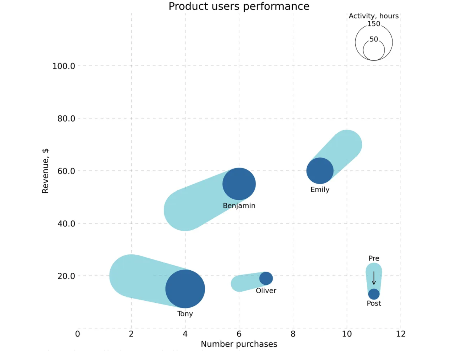
plt.textual content(legend_position[0], legend_position[1] + 2*legend_label_r + 0.3, 'Exercise, hours', fontsize=12, ha="middle", va="middle")

Our closing chart seems like this:

The visualization seems very fashionable and concentrates numerous data in a compact kind.

Right here is the complete code for the graph:

import matplotlib.pyplot as plt
import numpy as np
import pandas as pd
import sympy as sp
from scipy.spatial import ConvexHull
import math
from matplotlib import rcParams
import matplotlib.patches as patches

def check_position_relative_to_line(a, b, x0, y0):
    y_line = a * x0 + b
    
    if y0 > y_line:
        return 1 # line is above the purpose
    elif y0 < y_line:
        return -1

    
def find_tangent_equations(x1, y1, r1, x2, y2, r2):
    a, b = sp.symbols('a b')

    tangent_1 = (a*x1 + b - y1)**2 - r1**2 * (a**2 + 1)  
    tangent_2 = (a*x2 + b - y2)**2 - r2**2 * (a**2 + 1) 

    eqs_1 = [tangent_2, tangent_1]
    answer = sp.clear up(eqs_1, (a, b))
    parameters = [(float(e[0]), float(e[1])) for e in answer]

    # filter simply exterior tangents
    parameters_filtered = []
    for tangent in parameters:
        a = tangent[0]
        b = tangent[1]
        if abs(check_position_relative_to_line(a, b, x1, y1) + check_position_relative_to_line(a, b, x2, y2)) == 2:
            parameters_filtered.append(tangent)

    return parameters_filtered

def find_circle_line_intersection(circle_x, circle_y, circle_r, line_a, line_b):
    x, y = sp.symbols('x y')
    circle_eq = (x - circle_x)**2 + (y - circle_y)**2 - circle_r**2
    intersection_eq = circle_eq.subs(y, line_a * x + line_b)

    sol_x_raw = sp.clear up(intersection_eq, x)[0]
    attempt:
        sol_x = float(sol_x_raw)
    besides:
        sol_x = sol_x_raw.as_real_imag()[0]
    sol_y = line_a * sol_x + line_b
    return sol_x, sol_y

def draw_polygon(plt, factors):
    hull = ConvexHull(factors)
    convex_points = [points[i] for i in hull.vertices]

    x, y = zip(*convex_points)
    x += (x[0],)
    y += (y[0],)

    plt.fill(x, y, colour="#99d8e1", alpha=1, zorder=1)

def area_to_radius(space):
    radius = math.sqrt(space / math.pi)
    return radius

# information technology
df = pd.DataFrame({'consumer': ['Emily', 'Emily', 'James', 'James', 'Tony', 'Tony', 'Olivia', 'Olivia', 'Oliver', 'Oliver', 'Benjamin', 'Benjamin'],
                   'interval': ['pre', 'post', 'pre', 'post', 'pre', 'post', 'pre', 'post', 'pre', 'post', 'pre', 'post'],
                   'num_purchases': [10, 9, 3, 5, 2, 4, 8, 7, 6, 7, 4, 6],
                   'income': [70, 60, 80, 90, 20, 15, 80, 76, 17, 19, 45, 55],
                   'exercise': [100, 80, 50, 90, 210, 170, 60, 55, 30, 20, 200, 120]})

x_alias, y_alias, a_alias="num_purchases", 'income', 'exercise'

# scaling metrics
radius_scaler = 0.1
df['radius'] = df[a_alias].apply(area_to_radius) * radius_scaler
df['y_scaled'] = df[y_alias] / df[x_alias].max()

# plot parameters
plt.subplots(figsize=(10, 10))
rcParams['font.family'] = 'DejaVu Sans'
rcParams['font.size'] = 14
plt.grid(colour="grey", linestyle=(0, (10, 10)), linewidth=0.5, alpha=0.6, zorder=1)
plt.axvline(x=0, colour="white", linewidth=2)
plt.gca().set_facecolor('white')
plt.gcf().set_facecolor('white')

# spines formatting
plt.gca().spines["top"].set_visible(False)
plt.gca().spines["right"].set_visible(False)
plt.gca().spines["bottom"].set_visible(False)
plt.gca().spines["left"].set_visible(False)
plt.gca().tick_params(axis="each", which="each", size=0)

# plot labels
plt.xlabel("Quantity purchases") 
plt.ylabel("Income, $")
plt.title("Product customers efficiency", fontsize=18, colour="black")

# axis limits
axis_lim = df[x_alias].max() * 1.2
plt.xlim(0, axis_lim)
plt.ylim(0, axis_lim)

# bubble pre
for _, row in df[df.period=='pre'].iterrows():
    x = row[x_alias]
    y = row.y_scaled
    r = row.radius
    circle = patches.Circle((x, y), r, facecolor="#99d8e1", edgecolor="none", linewidth=0, zorder=2)
    plt.gca().add_patch(circle)

# transition space
for consumer in df.consumer.distinctive():
    user_pre = df[(df.user==user) & (df.period=='pre')]
    x1, y1, r1 = user_pre[x_alias].values[0], user_pre.y_scaled.values[0], user_pre.radius.values[0]
    user_post = df[(df.user==user) & (df.period=='post')]
    x2, y2, r2 = user_post[x_alias].values[0], user_post.y_scaled.values[0], user_post.radius.values[0]

    tangent_equations = find_tangent_equations(x1, y1, r1, x2, y2, r2)
    circle_1_line_intersections = [find_circle_line_intersection(x1, y1, r1, eq[0], eq[1]) for eq in tangent_equations]
    circle_2_line_intersections = [find_circle_line_intersection(x2, y2, r2, eq[0], eq[1]) for eq in tangent_equations]

    polygon_points = circle_1_line_intersections + circle_2_line_intersections
    draw_polygon(plt, polygon_points)

# bubble put up
for _, row in df[df.period=='post'].iterrows():
    x = row[x_alias]
    y = row.y_scaled
    r = row.radius
    label = row.consumer
    circle = patches.Circle((x, y), r, facecolor="#2d699f", edgecolor="none", linewidth=0, zorder=2)
    plt.gca().add_patch(circle)

    plt.textual content(x, y - r - 0.3, label, fontsize=12, ha="middle")

# bubble measurement legend
legend_areas_original = [150, 50]
legend_position = (11, 10.2)
for i in legend_areas_original:
    i_r = area_to_radius(i) * radius_scaler
    circle = plt.Circle((legend_position[0], legend_position[1] + i_r), i_r, colour="black", fill=False, linewidth=0.6, facecolor="none")
    plt.gca().add_patch(circle)
    plt.textual content(legend_position[0], legend_position[1] + 2*i_r, str(i), fontsize=12, ha="middle", va="middle",
              bbox=dict(facecolor="white", edgecolor="none", boxstyle="spherical,pad=0.1"))
legend_label_r = area_to_radius(np.max(legend_areas_original)) * radius_scaler
plt.textual content(legend_position[0], legend_position[1] + 2*legend_label_r + 0.3, 'Exercise, hours', fontsize=12, ha="middle", va="middle")


## pre-post legend 
# circle 1
legend_position, r1 = (11, 2.2), 0.3
x1, y1 = legend_position[0], legend_position[1]
circle = patches.Circle((x1, y1), r1, facecolor="#99d8e1", edgecolor="none", linewidth=0, zorder=2)
plt.gca().add_patch(circle)
plt.textual content(x1, y1 + r1 + 0.15, 'Pre', fontsize=12, ha="middle", va="middle")
# circle 2
x2, y2 = legend_position[0], legend_position[1] - r1*3
r2 = r1*0.7
circle = patches.Circle((x2, y2), r2, facecolor="#2d699f", edgecolor="none", linewidth=0, zorder=2)
plt.gca().add_patch(circle)
plt.textual content(x2, y2 - r2 - 0.15, 'Submit', fontsize=12, ha="middle", va="middle")
# tangents
tangent_equations = find_tangent_equations(x1, y1, r1, x2, y2, r2)
circle_1_line_intersections = [find_circle_line_intersection(x1, y1, r1, eq[0], eq[1]) for eq in tangent_equations]
circle_2_line_intersections = [find_circle_line_intersection(x2, y2, r2, eq[0], eq[1]) for eq in tangent_equations]
polygon_points = circle_1_line_intersections + circle_2_line_intersections
draw_polygon(plt, polygon_points)
# small arrow
plt.annotate('', xytext=(x1, y1), xy=(x2, y1 - r1*2), arrowprops=dict(edgecolor="black", arrowstyle="->", lw=1))

# y axis formatting
max_y = df[y_alias].max()
nearest_power_of_10 = 10 ** math.ceil(math.log10(max_y))
ticks = [round(nearest_power_of_10/5 * i, 2) for i in range(0, 6)]
yticks_scaled = ticks / df[x_alias].max()
yticklabels = [str(i) for i in ticks]
yticklabels[0] = ''
plt.yticks(yticks_scaled, yticklabels)

plt.savefig("plot_with_white_background.png", bbox_inches="tight", dpi=300)

Including a time dimension to bubble charts enhances their skill to convey dynamic information adjustments intuitively. By implementing easy transitions between “earlier than” and “after” states, customers can higher perceive developments and comparisons over time.

Whereas no ready-made options had been obtainable, growing a customized method proved each difficult and rewarding, requiring mathematical insights and cautious animation strategies. The proposed methodology could be simply prolonged to numerous datasets, making it a helpful device for Knowledge Visualization in enterprise, science, and analytics.