


Introduction
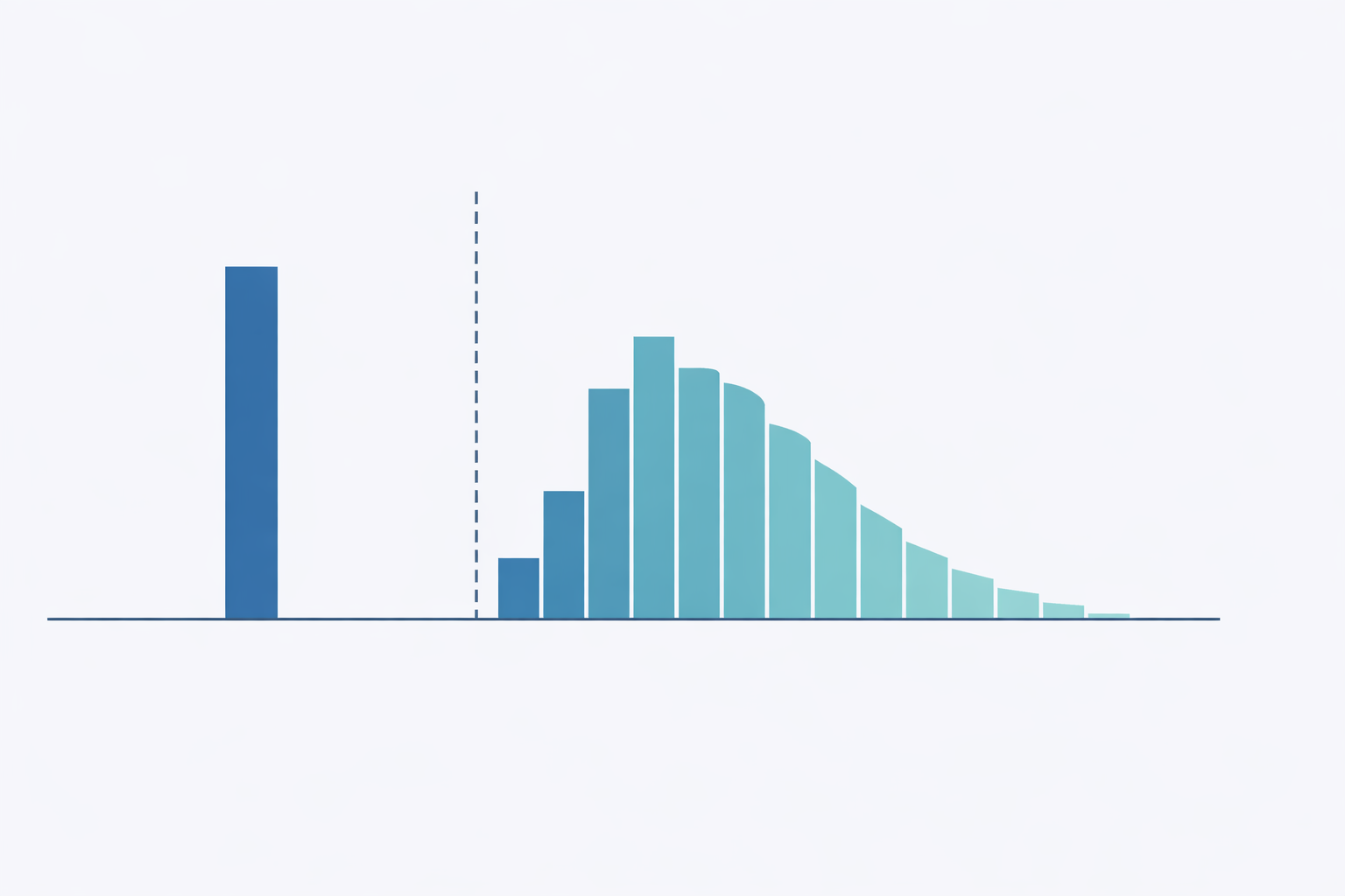
, we often encounter prediction issues the place the end result has an uncommon distribution: a big mass of zeros mixed with a steady or rely distribution for optimistic values. Should you’ve labored in any customer-facing area, you’ve virtually actually run into this. Take into consideration predicting buyer spending. In any given week, the overwhelming majority of customers in your platform don’t buy something in any respect, however the ones who do may spend anyplace from $5 to $5,000. Insurance coverage claims observe the same sample: most policyholders don’t file something in a given quarter, however the claims that do are available in range enormously in dimension. You see the identical construction in mortgage prepayments, worker turnover timing, advert click on income, and numerous different enterprise outcomes.
The intuition for many groups is to succeed in for the standard regression mannequin and attempt to make it work. I’ve seen this play out a number of occasions. Somebody suits an OLS mannequin, will get destructive predictions for half the shopper base, provides a ground at zero, and calls it a day. Or they struggle a log-transform, run into the $log(0)$ downside, tack on a $+1$ offset, and hope for the most effective. These workarounds may work, however they gloss over a elementary challenge: the zeros and the optimistic values in your knowledge are sometimes generated by fully completely different processes. A buyer who won’t ever purchase your product is essentially completely different from a buyer who buys often however occurred to not this week. Treating them the identical manner in a single mannequin forces the algorithm to compromise on each teams, and it often does a poor job on every.
The two-stage hurdle mannequin offers a extra principled answer by decomposing the issue into two distinct questions.
First, will the end result be zero or optimistic?
And second, provided that it’s optimistic, what is going to the worth be?
By separating the “if” from the “how a lot,” we are able to use the proper instruments on every sub-problem independently with completely different algorithms, completely different options, and completely different assumptions, then mix the outcomes right into a single prediction.
On this article, I’ll stroll via the speculation behind hurdle fashions, present a working Python implementation, and focus on the sensible issues that matter when deploying these fashions in manufacturing.
readers who’re already accustomed to the motivation can skip straight to the implementation part.
The Drawback with Customary Approaches
Why Not Simply Use Linear Regression? To make this concrete, take into account predicting buyer spend.
If 80% of consumers spend zero and the remaining 20% spend between 10 and 1000 {dollars}, a linear regression mannequin instantly runs into hassle.
The mannequin can (and can) predict destructive spend for some clients, which is nonsensical since you’ll be able to’t spend destructive {dollars}.
It’ll additionally wrestle on the boundary: the large spike at zero pulls the regression line down, inflicting the mannequin to underpredict zeros and overpredict small optimistic values concurrently.
The variance construction can also be incorrect.
Clients who spend nothing have zero variance by definition, whereas clients who do spend have excessive variance.
Whereas you should use heteroskedasticity-robust commonplace errors to get legitimate inference regardless of non-constant variance, that solely fixes the usual errors and doesn’t repair the predictions themselves.
The fitted values are nonetheless coming from a linear mannequin that’s attempting to common over a spike at zero and a right-skewed optimistic distribution, which is a poor match no matter the way you compute the arrogance intervals.
Why Not Log-Remodel? The following factor most individuals attempt is a log-transform: $log(y + 1)$ or $log(y + epsilon)$.
This compresses the proper tail and makes the optimistic values look extra regular, but it surely introduces its personal set of issues.
The selection of offset ($1$ or $epsilon$) is unfair, and your predictions will change relying on what you decide.
While you back-transform by way of $exp(hat{y}) – 1$, you introduce a scientific bias attributable to Jensen’s inequality, because the anticipated worth of the exponentiated prediction is just not the identical because the exponentiation of the anticipated prediction.
Extra essentially, the mannequin nonetheless doesn’t distinguish between a buyer who by no means spends and one who typically spends however occurred to be zero this era.
Each get mapped to $log(0 + 1) = 0$, and the mannequin treats them identically although they signify very completely different buyer behaviors.
What This Means for Forecasting. The deeper challenge with forcing a single mannequin onto zero-inflated knowledge goes past poor level estimates.
While you ask one mannequin to explain two essentially completely different behaviors (not partaking in any respect vs. partaking at various intensities), you find yourself with a mannequin that conflates the drivers of every.
The options that predict whether or not a buyer will buy in any respect are sometimes fairly completely different from the options that predict how a lot they’ll spend given a purchase order.
Recency and engagement frequency may dominate the “will they purchase” query, whereas earnings and product class preferences matter extra for the “how a lot” query.
A single regression mixes these alerts collectively, making it tough to disentangle what’s really driving the forecast.
This additionally has sensible implications for a way you act on the mannequin.
In case your forecast is low for a specific buyer, is it as a result of they’re unlikely to buy, or as a result of they’re more likely to buy however at a small quantity?
The optimum enterprise response to every situation is completely different.
You may ship a re-engagement marketing campaign for the primary case and an upsell provide for the second.
A single mannequin provides you one quantity, however there isn’t any strategy to inform which lever to drag.
The Two-Stage Hurdle Mannequin
Conceptual Framework. The core thought behind hurdle fashions is surprisingly intuitive.
Zeros and positives typically come up from completely different data-generating processes, so we should always mannequin them individually.
Consider it as two sequential questions your mannequin must reply.
First, does this buyer cross the “hurdle” and interact in any respect?
And second, provided that they’ve engaged, how a lot do they spend?
Formally, we are able to write the distribution of the end result $Y$ conditional on options $X$ as:
$$ P(Y = y | X) = start{instances} 1 – pi(X) & textual content{if } y = 0 pi(X) cdot f(y | X, y > 0) & textual content{if } y > 0 finish{instances} $$
Right here, $pi(X)$ is the likelihood of crossing the hurdle (having a optimistic final result), and $f(y | X, y > 0)$ is the conditional distribution of $y$ provided that it’s optimistic.
The fantastic thing about this formulation is that these two elements will be modeled independently.
You should utilize a gradient boosting classifier for the primary stage and a gamma regression for the second, or logistic regression paired with a neural community, or some other mixture that fits your knowledge.
Every stage will get its personal function set, its personal hyperparameters, and its personal analysis metrics.
This modularity is what makes hurdle fashions so sensible in manufacturing settings.
Stage 1: The Classification Mannequin. The primary stage is an easy binary classification downside: predict whether or not $y > 0$.
You’re coaching on the total dataset, with each commentary labeled as both zero or optimistic.
This can be a downside that the ML neighborhood has many years of tooling for.
Logistic regression provides you an interpretable and quick baseline.
Gradient boosting strategies like XGBoost or LightGBM deal with non-linearities and have interactions nicely.
Neural networks work when you might have high-dimensional or unstructured options.
The output from this stage is $hat{pi}(X) = P(Y > 0 | X)$, a calibrated likelihood that the end result can be optimistic.
The vital factor to get proper right here is calibration.
Since we’re going to multiply this likelihood by the conditional quantity within the subsequent stage, we’d like $hat{pi}(X)$ to be a real likelihood, not only a rating that ranks nicely.
In case your classifier outputs possibilities which might be systematically too excessive or too low, the mixed prediction will inherit that bias.
Platt scaling may also help in case your base classifier isn’t well-calibrated out of the field.
Stage 2: The Conditional Regression Mannequin. The second stage predicts the worth of $y$ conditional on $y > 0$.
That is the place the hurdle mannequin shines in comparison with commonplace approaches since you’re coaching a regression mannequin completely on the optimistic subset of your knowledge, so the mannequin by no means has to cope with the spike at zero.
This implies you should use the total vary of regression strategies with out worrying about how they deal with zeros.
The selection of mannequin for this stage relies upon closely on the form of your optimistic outcomes.
If $log(y | y > 0)$ is roughly regular, you should use OLS on the log-transformed goal (with applicable bias correction on back-transformation, which we’ll cowl under).
For right-skewed optimistic steady outcomes, a GLM with a gamma household is a pure alternative.
Should you’re coping with overdispersed rely knowledge, destructive binomial regression works nicely.
A straightforward technique is simply to make use of Autogluon because the ensemble mannequin and never have to fret concerning the distribution of your knowledge.
The output is $hat{mu}(X) = E[Y | X, Y > 0]$, the anticipated worth conditional on the end result being optimistic.
Mixed Prediction. The ultimate prediction combines each phases multiplicatively:
$$ hat{E}[Y | X] = hat{pi}(X) cdot hat{mu}(X) $$
This offers the unconditional anticipated worth of $Y$, accounting for each the likelihood that the end result is optimistic and the anticipated magnitude given positivity.
If a buyer has a 30% probability of buying and their anticipated spend given a purchase order is 100 {dollars}, then their unconditional anticipated spend is 30 {dollars}.
This decomposition additionally makes enterprise interpretation easy.
You may individually get hold of function significance on each the likelihood of engagement versus what drives the depth of engagement to see what must be addressed.
Implementation
Coaching Pipeline. The coaching pipeline is easy.
We practice Stage 1 on the total dataset with a binary goal, then practice Stage 2 on solely the optimistic observations with the unique steady goal.
At prediction time, we get a likelihood from Stage 1 and a conditional imply from Stage 2, then multiply them collectively.

We are able to implement this in Python utilizing scikit-learn as a place to begin.
The next class wraps each phases right into a single estimator that follows the scikit-learn API, making it straightforward to drop into present pipelines and use with instruments like cross-validation and grid search.
import numpy as np
from sklearn.linear_model import LogisticRegression
from sklearn.ensemble import GradientBoostingRegressor
from sklearn.base import BaseEstimator, RegressorMixin

class HurdleModel(BaseEstimator, RegressorMixin):
    """
    Two-stage hurdle mannequin for zero-inflated steady outcomes.

    Stage 1: Binary classifier for P(Y > 0)
    Stage 2: Regressor for E[Y | Y > 0]
    """

    def __init__(self, classifier=None, regressor=None):
        self.classifier = classifier or LogisticRegression()
        self.regressor = regressor or GradientBoostingRegressor()

    def match(self, X, y):
        # Stage 1: Practice classifier on all knowledge
        y_binary = (y > 0).astype(int)
        self.classifier.match(X, y_binary)

        # Stage 2: Practice regressor on optimistic outcomes solely
        positive_mask = y > 0
        if positive_mask.sum() > 0:
            X_positive = X[positive_mask]
            y_positive = y[positive_mask]
            self.regressor.match(X_positive, y_positive)

        return self

    def predict(self, X):
        # P(Y > 0)
        prob_positive = self.classifier.predict_proba(X)[:, 1]

        # E[Y | Y > 0]
        conditional_mean = self.regressor.predict(X)

        # E[Y] = P(Y > 0) * E[Y | Y > 0]
        return prob_positive * conditional_mean

    def predict_proba_positive(self, X):
        """Return likelihood of optimistic final result."""
        return self.classifier.predict_proba(X)[:, 1]

    def predict_conditional(self, X):
        """Return anticipated worth given optimistic final result."""
        return self.regressor.predict(X)
Sensible Concerns
Function Engineering. One of many good properties of this framework is that the 2 phases can use fully completely different function units.
In my expertise, the options that predict whether or not somebody engages in any respect are sometimes fairly completely different from the options that predict how a lot they interact.
For Stage 1, behavioral alerts are likely to dominate: previous exercise, recency, frequency, whether or not the shopper has ever bought earlier than.
Demographic indicators and contextual elements like time of yr or day of week additionally assist separate the “will interact” group from the “gained’t interact” group.
For Stage 2, depth alerts matter extra: historic buy quantities, spending velocity, capability indicators like earnings or credit score restrict, and product or class preferences.
These options assist distinguish the 50 greenback spender from the five hundred greenback spender, conditional on each of them making a purchase order.
Moreover, we are able to use function boosting by feeding within the output of the stage 1 mannequin into the stage 2 mannequin as an extra function.
This permits the stage 2 mannequin to learn the way the likelihood of engagement interacts with the depth alerts, which improves efficiency.
Dealing with Class Imbalance. If zeros dominate your dataset, say 95% of observations are zero, then Stage 1 faces a category imbalance downside.
That is widespread in functions like advert clicks or insurance coverage claims.
The usual toolkit applies right here: you’ll be able to tune the classification threshold to optimize on your particular enterprise goal somewhat than utilizing the default 0.5 cutoff, upweight the minority class throughout coaching via pattern weights, or apply undersampling to resolve this.
The bottom line is to think twice about what you’re optimizing for.
In lots of enterprise settings, you care extra about precision on the high of the ranked checklist than you do about total accuracy, and tuning your threshold accordingly could make a giant distinction.
Mannequin Calibration. For the reason that mixed prediction $hat{pi}(X) cdot hat{mu}(X)$ is a product of two fashions, each have to be well-calibrated for the ultimate output to be dependable.
If Stage 1’s possibilities are systematically inflated by 10%, your mixed predictions can be inflated by 10% throughout the board, no matter how good Stage 2 is.
For Stage 1, examine calibration curves and apply Platt scaling if the uncooked possibilities are off.
For Stage 2, confirm that the predictions are unbiased on the optimistic subset, which means the imply of your predictions ought to roughly match the imply of the actuals when evaluated on holdout knowledge the place $y > 0$.
I’ve discovered that calibration points in Stage 1 are the extra widespread supply of issues in apply, particularly when extending the classifier to a discrete-time hazard mannequin.
Analysis Metrics. Evaluating a two-stage mannequin requires enthusiastic about every stage individually after which trying on the mixed output.
For Stage 1, commonplace classification metrics apply: AUC-ROC and AUC-PR for rating high quality, precision and recall at your chosen threshold for operational efficiency, and the Brier rating for calibration.
For Stage 2, it’s best to consider solely on the optimistic subset since that’s what the mannequin was educated on.
RMSE and MAE offer you a way of absolute error, MAPE tells you about share errors (which issues when your outcomes span a number of orders of magnitude), and quantile protection tells you whether or not your prediction intervals are sincere.
For the mixed mannequin, take a look at total RMSE and MAE on the total take a look at set, but additionally break it down by whether or not the true final result was zero or optimistic.
A mannequin that appears nice on combination is likely to be horrible at one finish of the distribution.
Raise charts by predicted decile are additionally helpful for speaking mannequin efficiency to stakeholders who don’t assume by way of RMSE.
When to Use Hurdle vs. Zero-Inflated Fashions. This can be a distinction value getting proper, as a result of hurdle fashions and zero-inflated fashions (like ZIP or ZINB) make completely different assumptions about the place the zeros come from.
Hurdle fashions assume that every one zeros come up from a single course of, the “non-participation” course of.
When you cross the hurdle, you’re within the optimistic regime, and the zeros are totally defined by Stage 1.
Zero-inflated fashions, alternatively, assume that zeros can come from two sources: some are “structural” zeros (clients who might by no means be optimistic, like somebody who doesn’t personal a automobile being requested about auto insurance coverage claims), and others are “sampling” zeros (clients who might have been optimistic however simply weren’t this time).
To make this concrete with a retail instance: a hurdle mannequin says a buyer both decides to buy or doesn’t, and in the event that they store, they spend some optimistic quantity.
A zero-inflated mannequin says some clients by no means store at this retailer (structural zeros), whereas others do store right here often however simply didn’t at the moment (sampling zeros).
In case your zeros genuinely come from two distinct populations, a zero-inflated mannequin is extra applicable.
However in lots of sensible settings, the hurdle framing is each easier and adequate, and I’d suggest beginning there except you might have a transparent motive to imagine in two sorts of zeros.
Extensions and Variations
Multi-Class Hurdle. Typically the binary cut up between zero and optimistic isn’t granular sufficient.
In case your final result has a number of significant states (say none, small, and enormous), you’ll be able to prolong the hurdle framework right into a multi-class model.
The primary stage turns into a multinomial classifier that assigns every commentary to considered one of $Okay$ buckets, after which separate regression fashions deal with every bucket’s conditional distribution.
Formally, this seems like:
$$ P(Y) = start{instances} pi_0 & textual content{if } Y = 0 pi_1 cdot f_{textual content{small}}(Y) & textual content{if } 0 < Y leq tau pi_2 cdot f_{textual content{massive}}(Y) & textual content{if } Y > tau finish{instances} $$
That is notably helpful when the optimistic outcomes themselves have distinct sub-populations.
As an example, in modeling insurance coverage claims, there’s typically a transparent separation between small routine claims and enormous catastrophic ones, and attempting to suit a single distribution to each results in poor tail estimates.
The edge $tau$ will be set based mostly on area information or estimated from the information utilizing combination mannequin strategies.
Generalizing the Phases. One factor value emphasizing is that neither stage must be a particular sort of mannequin.
All through this text, I’ve introduced Stage 1 as a binary classifier, however that’s simply the only model.
If the timing of the occasion issues, you can exchange Stage 1 with a discrete-choice survival mannequin that predicts not simply whether or not a buyer will buy, however when.
That is particularly helpful for subscription or retention contexts the place the “hurdle” has a temporal dimension.
Equally, Stage 2 doesn’t must be a single hand-tuned regression.
You would use an AutoML framework like AutoGluon to ensemble over a big set of candidate fashions (gradient boosting, neural networks, linear fashions) and let it discover the most effective mixture for predicting the conditional quantity.
The hurdle framework is agnostic to what sits inside every stage, so it’s best to be happy to swap in no matter modeling method most closely fits your knowledge and use case.
Frequent Pitfalls
These are errors I’ve both made myself or seen others make when deploying hurdle fashions.
None of them are apparent till you’ve been bitten, so that they’re value studying via even when you’re already comfy with the framework.
1. Leaking Stage 2 Info into Stage 1. Should you engineer options from the goal, one thing like “common historic spend” or “complete lifetime worth,” you should watch out about how that info flows into every stage.
A function that summarizes previous spend implicitly incorporates details about whether or not the shopper has ever spent something, which suggests Stage 1 is likely to be getting a free sign that wouldn’t be obtainable at prediction time for brand new clients.
The repair is to think twice concerning the temporal construction of your options and ensure each phases solely see info that will be obtainable on the time of prediction.
2. Ignoring the Conditional Nature of Stage 2. This one is delicate however vital.
Stage 2 is educated solely on observations the place $y > 0$, so it needs to be evaluated solely on that subset too.
I’ve seen individuals compute RMSE throughout the total take a look at set (together with zeros) and conclude that Stage 2 is horrible.
So once you’re reporting metrics for Stage 2, at all times filter to the optimistic subset first.
Equally, when diagnosing points with the mixed mannequin, be sure to decompose the error into its Stage 1 and Stage 2 elements.
A excessive total error is likely to be pushed fully by poor classification in Stage 1, even when Stage 2 is doing high quality on the optimistic observations.
4. Misaligned Practice/Take a look at Splits. Each phases want to make use of the identical practice/take a look at splits.
This sounds apparent, but it surely’s straightforward to mess up in apply, particularly when you’re coaching the 2 phases in separate notebooks or pipelines.
If Stage 1 sees a buyer in coaching however Stage 2 sees the identical buyer in its take a look at set (since you re-split the positive-only knowledge independently), you’ve launched knowledge leakage.
The only repair is to do your practice/take a look at cut up as soon as originally on the total dataset, after which derive the Stage 2 coaching knowledge by filtering the coaching fold to optimistic observations.
Should you’re doing cross-validation, the fold assignments should be constant throughout each phases.
5.
Assuming Independence Between Phases. Whereas we mannequin the 2 phases individually, the underlying options and outcomes are sometimes correlated in ways in which matter.
Clients with excessive $hat{pi}(X)$ (more likely to interact) typically even have excessive $hat{mu}(X)$ (probably to spend so much once they do).
This implies the multiplicative mixture $hat{pi}(X) cdot hat{mu}(X)$ can amplify errors in methods you wouldn’t see if the phases had been actually impartial.
Hold this in thoughts when deciphering function significance.
A function that reveals up as vital in each phases is doing double responsibility, and its complete contribution to the mixed prediction is bigger than both stage’s significance rating suggests.
Last Remarks
Alternate Makes use of: Past the examples lined on this article, hurdle fashions present up in a shocking number of enterprise contexts.
In advertising, they’re a pure match for modeling buyer lifetime worth, the place many shoppers churn earlier than making a second buy, making a mass of zeros, whereas retained clients generate extensively various quantities of income.
In healthcare analytics, affected person value modeling follows the identical sample: most sufferers have zero claims in a given interval, however the claims that do are available in vary from routine workplace visits to main surgical procedures.
For demand forecasting with intermittent demand patterns (spare components, luxurious items, B2B transactions), the two-stage decomposition naturally captures the sporadic nature of purchases and avoids the smoothing artifacts that plague conventional time collection strategies.
In credit score danger, anticipated loss calculations are inherently a hurdle downside: what’s the likelihood of default (Stage 1), and what’s the loss given default (Stage 2)?
Should you’re working with any final result the place zeros have a essentially completely different which means than “only a small worth,” hurdle fashions are value contemplating as a primary method.
Two-stage hurdle fashions present a principled method to predicting zero-inflated outcomes by decomposing the issue into two conceptually distinct components: whether or not an occasion happens and what magnitude it takes conditional on incidence.
This decomposition gives flexibility, since every stage can use completely different algorithms, options, and tuning methods.
It gives interpretability, as a result of you’ll be able to individually analyze and current what drives participation versus what drives depth, which is usually precisely the breakdown that product managers and executives wish to see.
And it typically delivers higher predictive efficiency than a single mannequin attempting to deal with each the spike at zero and the continual optimistic distribution concurrently.
The important thing perception is recognizing that zeros and optimistic values typically come up from completely different mechanisms, and modeling them individually respects that construction somewhat than combating in opposition to it.
Whereas this text covers the core framework, we haven’t touched on a number of different vital extensions that deserve their very own remedy.
Bayesian formulations of hurdle fashions can incorporate prior information and supply pure uncertainty quantification, which might tie in properly with our hierarchical Bayesian collection.
Think about estimating product-level hurdle fashions the place merchandise with sparse knowledge borrow energy from their class.
Deep studying approaches open up the opportunity of utilizing unstructured options (textual content, photos) in both stage.
You probably have the chance to use hurdle fashions in your personal work, I’d love to listen to about it!
Please don’t hesitate to succeed in out with questions, insights, or tales via my electronic mail or LinkedIn.
You probably have any suggestions on this text, or want to request one other subject in causal inference/machine studying, please additionally be happy to succeed in out.
Thanks for studying!


