


5 days of this Machine Studying “Creation Calendar”, we explored 5 fashions (or algorithms) which are all primarily based on distances (native Euclidean distance, or world Mahalanobis distance).
So it’s time to change the strategy, proper? We’ll come again to the notion of distance later.
For at the moment, we are going to see one thing completely completely different: Choice Bushes!

Introduction with a Easy dataset
Let’s use a easy dataset with just one steady characteristic.
As all the time, the thought is you could visualize the outcomes your self. Then you need to suppose the way to make the pc do it.

We will visually guess that for the primary break up, there are two doable values, one round 5.5 and the opposite round 12.
Now the query is, which one will we select?
That is precisely what we’re going to discover out: how will we decide the worth for the primary break up with an implementation in Excel?
As soon as we decide the worth for the primary break up, we are able to apply the identical course of for the next splits.
That’s the reason we are going to solely implement the primary break up in Excel.
The Algorithmic Precept of Choice Tree Regressors
I wrote an article to all the time distinguish three steps of machine studying to be taught it successfully, and let’s apply the precept to Choice Tree Regressors.
So for the primary time, now we have a “true” machine studying mannequin, with non-trivial steps for all three.
What’s the mannequin?
The mannequin here’s a algorithm, to partition the dataset, and for every partition, we’re going to assign a price. Which one? The common worth y of all of the observations in the identical group.
So whereas k-NN predicts with the common worth of the closest neighbors (related observations when it comes to options variables), the Choice Tree regressor predicts with the common worth of a bunch of observations (related when it comes to the characteristic variable).
Mannequin becoming or coaching course of
For a call tree, we additionally name this course of absolutely rising a tree. Within the case of a Choice Tree Regressor, the leaves will comprise just one remark, with thus a MSE of zero.
Rising a tree consists of recursively partitioning the enter knowledge into smaller and smaller chunks or areas. For every area, a prediction could be calculated.
Within the case of regression, the prediction is the common of the goal variable for the area.
At every step of the constructing course of, the algorithm selects the characteristic and the break up worth that maximizes the one criterion, and within the case of a regressor, it’s typically the Imply Squared Error (MSE) between the precise worth and the prediction.
Mannequin Tuning or Pruning
For a call tree, the final time period of mannequin tuning can be name it pruning, be it may be seen as dropping nodes and leaves from a completely grown tree.
It is usually equal to say that the constructing course of stops when a criterion is met, resembling a most depth or a minimal variety of samples in every leaf node. And these are the hyperparameters that may be optimized with the tuning course of.
Inferencing course of
As soon as the choice tree regressor is constructed, it may be used to foretell the goal variable for brand new enter cases by making use of the foundations and traversing the tree from the basis node to a leaf node that corresponds to the enter’s characteristic values.
The anticipated goal worth for the enter occasion is then the imply of the goal values of the coaching samples that fall into the identical leaf node.
Break up with One Steady Function
Listed below are the steps we are going to comply with:
- Listing all doable splits
- For every break up, we are going to calculate the MSE (Imply Squared Error)
- We’ll choose the break up that minimizes the MSE because the optimum subsequent break up
All doable splits
First, now we have to record all of the doable splits which are the common values of two consecutive values. There is no such thing as a want to check extra values.

MSE calculation for every doable break up
As a place to begin, we are able to calculate the MSE earlier than any splits. This additionally implies that the prediction is simply the common worth of y. And the MSE is equal to the Customary Deviation of y.
Now, the thought is to discover a break up in order that the MSE with a break up is decrease than earlier than. It’s doable that the break up doesn’t considerably enhance the efficiency (or decrease the MSE), then the ultimate tree could be trivial, that’s the common worth of y.
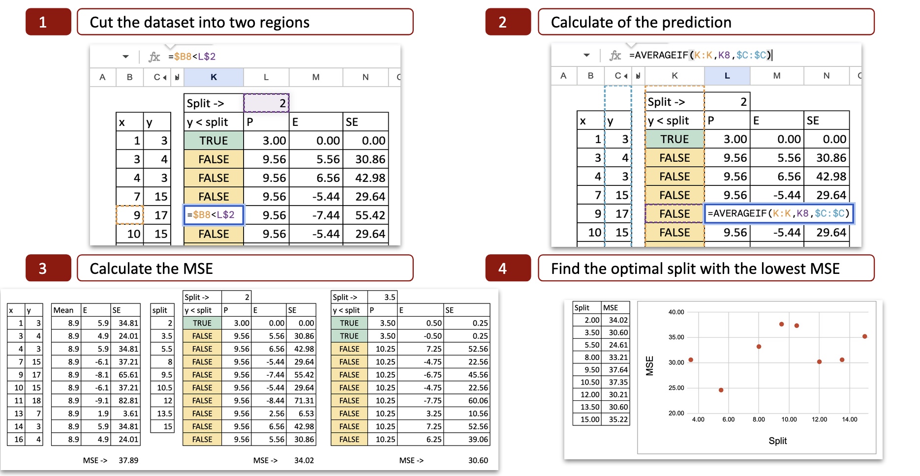
For every doable break up, we are able to then calculate the MSE (Imply Squared Error). The picture under reveals the calculation for the primary doable break up, which is x = 2.

We will see the main points of the calculation:
- Lower the dataset into two areas: with the worth x=2, we decide two potentialities x<2 or x>2, so the x axis is minimize into two components.
- Calculate the prediction: for every half, we calculate the common of y. That’s the potential prediction for y.
- Calculate the error: then we examine the prediction to the precise worth of y
- Calculate the squared error: for every remark, we are able to calculate the sq. error.

Optimum break up
For every doable break up, we do the identical to acquire the MSE. In Excel, we are able to copy and paste the system and the one worth that modifications is the doable break up worth for x.

Then we are able to plot the MSE on the y-axis and the doable break up on the x-axis, and now we are able to see that there’s a minimal of MSE for x=5.5, that is precisely the end result obtained with python code.

Now, one small train you are able to do is change the MSE to MAE (Imply Absolute Error).
And you may attempt to reply this query: what’s the impression of this variation?
Condensing All Break up Calculations into One Abstract Desk
Within the earlier sections, we computed every break up step-by-step, in order that we are able to higher visualize the main points of calculations.
Now we put all the things collectively in a single single desk, so the entire course of turns into compact and simple to automate.
To do that, we first simplify the calculations.
In a node, the prediction is the common, so the MSE is strictly the variance. And for the variance, we are able to additionally use the simplified system:

So within the following desk, we use one row for every doable break up.
For every break up, we calculate the MSE of the left node and the MSE of the correct node.
The variance of every group could be simplified utilizing the intermediate outcomes of y and y squared.
Then we compute the weighted common of the 2 MSE values. And in the long run, we get precisely the identical end result as within the step-by-step methodology.

Break up with A number of Steady Options
Now we are going to use two options.
That is the place it turns into attention-grabbing.
We could have candidate splits coming from each options.
How will we select?
We’ll merely contemplate all of them, after which choose the break up with the smallest MSE.
The concept in Excel is:
- first, put all doable splits from the 2 options into one single column,
- then, for every of those splits, calculate the MSE like earlier than,
- lastly, choose one of the best one.
Splits concatenation
First, we record all doable splits for Function 1 (for instance, all thresholds between two sorted values).
Then, we record all doable splits for Function 2 in the identical approach.
In Excel, we concatenate these two lists into one column of candidate splits.
So every row on this column represents:
- “If I minimize right here, utilizing this characteristic, what occurs to the MSE?”
This provides us one unified record of all splits from each options.

MSE calculations
As soon as now we have the record of all splits, the remainder is similar logic as earlier than.
For every row (that’s, for every break up):
- we divide the factors into left node and proper node,
- we compute the MSE of the left node,
- we compute the MSE of the correct node,
- we take the weighted common of the 2 MSE values.
On the finish, we have a look at this column of “Whole MSE” and we select the break up (and due to this fact the characteristic and threshold) that offers the minimal worth.

Break up with One Steady and One Categorical Function
Now allow us to mix two very various kinds of options:
- one steady characteristic
- one categorical characteristic (for instance, A, B, C).
A choice tree can break up on each, however the best way we generate candidate splits will not be the identical.
With a steady characteristic, we check thresholds.
With a categorical characteristic, we check teams of classes.
So the thought is strictly the identical as earlier than:
we contemplate all doable splits from each options, then we choose the one with the smallest MSE.
Categorical characteristic splits
For a categorical characteristic, the logic is completely different:
- every class is already a “group”,
- so the only break up is: one class vs all of the others.
For instance, if the classes are A, B, and C:
- break up 1: A vs (B, C)
- break up 2: B vs (A, C)
- break up 3: C vs (A, B)
This already provides significant candidate splits and retains the Excel formulation manageable.
Every of those category-based splits is added to the identical record that incorporates the continual thresholds.
MSE calculation
As soon as all splits are listed (steady thresholds + categorical partitions), the calculations comply with the identical steps:
- assign every level to the left or proper node,
- compute the MSE of the left node,
- compute the MSE of the correct node,
- compute the weighted common.
The break up with the lowest complete MSE turns into the optimum first break up.

Train you possibly can check out
Now, you possibly can play with the Google Sheet:
- You’ll be able to attempt to discover the following break up
- You’ll be able to change the criterion, as a substitute of MSE, you should use absolute error, Poisson or friedman_mse as indicated within the documentation of DecisionTreeRegressor
- You’ll be able to change the goal variable to a binary variable, usually, this turns into a classification process, however 0 or 1 are additionally numbers so the criterion MSE nonetheless could be utilized. However if you wish to create a correct classifier, you need to apply the same old criterion Entroy or Gini. It’s for the following article.
Conclusion
Utilizing Excel, it’s doable to implement one break up to realize extra insights into how Choice Tree Regressors work. Despite the fact that we didn’t create a full tree, it’s nonetheless attention-grabbing, since an important half is discovering the optimum break up amongst all doable splits.
Yet another factor about lacking values
Have you ever observed one thing attention-grabbing about how options are dealt with between distance-based fashions, and resolution timber?
For distance-based fashions, all the things should be numeric. Steady options keep steady, and categorical options should be remodeled into numbers. The mannequin compares factors in area, so all the things has to reside on a numeric axis.
Choice Bushes do the inverse: they minimize options into teams. A steady characteristic turns into intervals. A categorical characteristic stays categorical.
And a lacking worth? It merely turns into one other class. There is no such thing as a have to impute first. The tree can naturally deal with it by sending all “lacking” values to 1 department, similar to some other group.


