Survival Evaluation When No One Dies: A Worth-Based mostly Strategy

is a statistical method used to reply the query: “How lengthy will one thing final?” That “one thing” might vary from a affected person’s lifespan to the sturdiness of a machine element or the period of a consumer’s subscription.

One of the crucial broadly used instruments on this space is the Kaplan-Meier estimator.

Born on the planet of biology, Kaplan-Meier made its debut monitoring life and dying. However like all true celeb algorithm, it didn’t keep in its lane. As of late, it’s displaying up in enterprise dashboards, advertising and marketing groups, and churn analyses in every single place.

However right here’s the catch: enterprise isn’t biology. It’s messy, unpredictable, and filled with plot twists. That is why there are a few points that make our lives tougher once we attempt to use survival evaluation within the enterprise world.

To start with, we’re sometimes not simply fascinated with whether or not a buyer has “survived” (no matter survival might imply on this context), however moderately in how a lot of that particular person’s financial worth has survived.

Secondly, opposite to biology, it’s very potential for purchasers to “die” and “resuscitate” a number of occasions (consider if you unsubscribe/resubscribe to an internet service).

On this article, we’ll see how one can lengthen the classical Kaplan-Meier method in order that it higher fits our wants: modeling a steady (financial) worth as a substitute of a binary one (life/dying) and permitting “resurrections”.

A refresher on the Kaplan-Meier estimator

Let’s pause and rewind for a second. Earlier than we begin customizing Kaplan-Meier to suit our enterprise wants, we want a fast refresher on how the traditional model works.

Suppose you had 3 topics (let’s say lab mice) and also you gave them a medication it’s essential take a look at. The medication was given at completely different moments in time: topic a acquired it in January, topic b in April, and topic c in Could.

Then, you measure how lengthy they survive. Topic a died after 6 months, topic c after 4 months, and topic b remains to be alive on the time of the evaluation (November).

Graphically, we will signify the three topics as follows:

Now, even when we wished to measure a easy metric, like common survival, we’d face an issue. In reality, we don’t understand how lengthy topic b will survive, as it’s nonetheless alive at this time.

This can be a classical drawback in statistics, and it’s known as “proper censoring“.

Proper censoring is stats-speak for “we don’t know what occurred after a sure level” and it’s a giant deal in survival evaluation. So large that it led to the event of one of the crucial iconic estimators in statistical historical past: the Kaplan-Meier estimator, named after the duo who launched it again within the Fifties.

So, how does Kaplan-Meier deal with our drawback?

First, we align the clocks. Even when our mice have been handled at completely different occasions, what issues is time since therapy. So we reset the x-axis to zero for everybody — day zero is the day they bought the drug.

Now that we’re all on the identical timeline, we need to construct one thing helpful: an mixture survival curve. This curve tells us the chance {that a} typical mouse in our group will survive not less than x months post-treatment.

Let’s observe the logic collectively.

• As much as time 3? Everybody’s nonetheless alive. So survival = 100%. Simple.
• At time 4, mouse c dies. Which means out of the three mice, solely 2 of them survived after time 4. That offers us a survival fee of 67% at time 4.
• Then at time 6, mouse a checks out. Of the two mice that had made it to time 6, just one survived, so the survival fee from time 5 to six is 50%. Multiply that by the earlier 67%, and we get 33% survival as much as time 6.
• After time 7 we don’t produce other topics which might be noticed alive, so the curve has to cease right here.

Let’s plot these outcomes:

Since code is usually simpler to know than phrases, let’s translate this to Python. We’ve the next variables:

• kaplan_meier, an array containing the Kaplan-Meier estimates for every time limit, e.g. the chance of survival as much as time t.
• obs_t, an array that tells us whether or not a person is noticed (e.g., not right-censored) at time t.
• surv_t, boolean array that tells us whether or not every particular person is alive at time t.
• surv_t_minus_1, boolean array that tells us whether or not every particular person is alive at time t-1.

All we’ve got to do is to take all of the people noticed at t, compute their survival fee from t-1 to t (survival_rate_t), and multiply it by the survival fee as much as time t-1 (km[t-1]) to acquire the survival fee as much as time t (km[t]). In different phrases,

survival_rate_t = surv_t[obs_t].sum() / surv_t_minus_1[obs_t].sum()

kaplan_meier[t] = kaplan_meier[t-1] * survival_rate_t

the place, in fact, the start line is kaplan_meier[0] = 1.

For those who don’t need to code this from scratch, the Kaplan-Meier algorithm is offered within the Python library lifelines, and it may be used as follows:

from lifelines import KaplanMeierFitter

KaplanMeierFitter().match(
    durations=[6,7,4],
    event_observed=[1,0,1],
).survival_function_["KM_estimate"]

For those who use this code, you’ll receive the identical outcome we’ve got obtained manually with the earlier snippet.

Thus far, we’ve been hanging out within the land of mice, drugs, and mortality. Not precisely your common quarterly KPI evaluation, proper? So, how is this handy in enterprise?

Transferring to a enterprise setting

Thus far, we’ve handled “dying” as if it’s apparent. In Kaplan-Meier land, somebody both lives or dies, and we will simply log the time of dying. However now let’s stir in some real-world enterprise messiness.

What even is “dying” in a enterprise context?

It seems it’s not simple to reply this query, not less than for a few causes:

1. “Demise” just isn’t simple to outline. Let’s say you’re working at an e-commerce firm. You need to know when a consumer has “died”. Do you have to depend them as useless after they delete their account? That’s simple to trace… however too uncommon to be helpful. What if they only begin buying much less? However how a lot much less is useless? Per week of silence? A month? Two? You see the issue. The definition of “dying” is unfair, and relying on the place you draw the road, your evaluation would possibly inform wildly completely different tales.
2. “Demise” just isn’t everlasting. Kaplan-Meier has been conceived for organic functions through which as soon as a person is useless there isn’t a return. However in enterprise functions, resurrection just isn’t solely potential however fairly frequent. Think about a streaming service for which individuals pay a month-to-month subscription. It’s simple to outline “dying” on this case: it’s when customers cancel their subscriptions. Nonetheless, it’s fairly frequent that, a while after cancelling, they re-subscribe.

So how does all this play out in knowledge?

Let’s stroll via a toy instance. Say we’ve got a consumer on our e-commerce platform. Over the previous 10 months, right here’s how a lot they’ve spent:

To squeeze this into the Kaplan-Meier framework, we have to translate that spending conduct right into a life-or-death resolution.

So we make a rule: if a consumer stops spending for two consecutive months, we declare them “inactive”.

Graphically, this rule seems to be like the next:

Because the consumer spent $0 for 2 months in a row (month 4 and 5) we’ll take into account this consumer inactive ranging from month 4 on. And we’ll try this regardless of the consumer began spending once more in month 7. It is because, in Kaplan-Meier, resurrections are assumed to be unimaginable.

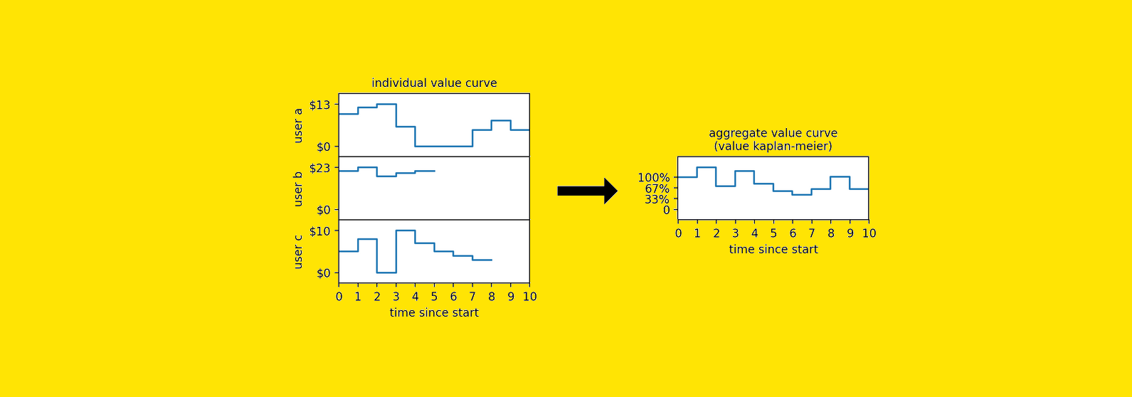
Now let’s add two extra customers to our instance. Since we’ve got determined a rule to show their worth curve right into a survival curve, we will additionally compute the Kaplan-Meier survival curve:

By now, you’ve most likely observed how a lot nuance (and knowledge) we’ve thrown away simply to make this work. Person a got here again from the useless — however we ignored that. Person c‘s spending dropped considerably — however Kaplan-Meier doesn’t care, as a result of all it sees is 1s and 0s. We pressured a steady worth (spending) right into a binary field (alive/useless), and alongside the way in which, we misplaced an entire lot of knowledge.

So the query is: can we lengthen Kaplan-Meier in a means that:

• retains the unique, steady knowledge intact,
• avoids arbitrary binary cutoffs,
• permits for resurrections?

Sure, we will. Within the subsequent part, I’ll present you ways.

Introducing “Worth Kaplan-Meier”

Let’s begin with the straightforward Kaplan-Meier method we’ve got seen earlier than.

# kaplan_meier: array containing the Kaplan-Meier estimates,
#               e.g. the chance of survival as much as time t
# obs_t: array, whether or not a topic has been noticed at time t
# surv_t: array, whether or not a topic was alive at time t
# surv_t_minus_1: array, whether or not a topic was alive at time t−1

survival_rate_t = surv_t[obs_t].sum() / surv_t_minus_1[obs_t].sum()

kaplan_meier[t] = kaplan_meier[t-1] * survival_rate_t

The primary change we have to make is to interchange surv_t and surv_t_minus_1, that are boolean arrays that inform us whether or not a topic is alive (1) or useless (0) with arrays that inform us the (financial) worth of every topic at a given time. For this objective, we will use two arrays named val_t and val_t_minus_1.

However this isn’t sufficient, as a result of since we’re coping with steady worth, each consumer is on a special scale and so, assuming that we need to weigh them equally, we have to rescale them based mostly on some particular person worth. However what worth ought to we use? Probably the most affordable selection is to make use of their preliminary worth at time 0, earlier than they have been influenced by no matter therapy we’re making use of to them.

So we additionally want to make use of one other vector, named val_t_0 that represents the worth of the person at time 0.

# value_kaplan_meier: array containing the Worth Kaplan-Meier estimates
# obs_t: array, whether or not a topic has been noticed at time t
# val_t_0: array, consumer worth at time 0
# val_t: array, consumer worth at time t
# val_t_minus_1: array, consumer worth at time t−1

value_rate_t = (
    (val_t[obs_t] / val_t_0[obs_t]).sum()
    / (val_t_minus_1[obs_t] / val_t_0[obs_t]).sum()
)

value_kaplan_meier[t] = value_kaplan_meier[t-1] * value_rate_t

What we’ve constructed is a direct generalization of Kaplan-Meier. In reality, if you happen to set val_t = surv_t, val_t_minus_1 = surv_t_minus_1, and val_t_0 as an array of 1s, this method collapses neatly again to our authentic survival estimator. So sure—it’s legit.

And right here is the curve that we’d receive when utilized to those 3 customers.

Let’s name this new model the Worth Kaplan-Meier estimator. In reality, it solutions the query:

How a lot % of worth remains to be surviving, on common, after x time?

We’ve bought the idea. However does it work within the wild?

Utilizing Worth Kaplan-Meier in apply

For those who take the Worth Kaplan-Meier estimator for a spin on real-world knowledge and examine it to the nice previous Kaplan-Meier curve, you’ll doubtless discover one thing comforting — they typically have the identical form. That’s an excellent signal. It means we haven’t damaged something basic whereas upgrading from binary to steady.

However right here’s the place issues get fascinating: Worth Kaplan-Meier normally sits a bit above its conventional cousin. Why? As a result of on this new world, customers are allowed to “resurrect”. Kaplan-Meier, being the extra inflexible of the 2, would’ve written them off the second they went quiet.

So how will we put this to make use of?

Think about you’re operating an experiment. At time zero, you begin a brand new therapy on a gaggle of customers. No matter it’s, you may monitor how a lot worth “survives” in each the therapy and management teams over time.

And that is what your output will most likely appear to be:

Conclusion

Kaplan-Meier is a broadly used and intuitive methodology for estimating survival features, particularly when the end result is a binary occasion like dying or failure. Nonetheless, many real-world enterprise eventualities contain extra complexity — resurrections are potential, and outcomes are higher represented by steady values moderately than a binary state.

In such circumstances, Worth Kaplan-Meier gives a pure extension. By incorporating the financial worth of people over time, it permits a extra nuanced understanding of worth retention and decay. This methodology preserves the simplicity and interpretability of the unique Kaplan-Meier estimator whereas adapting it to raised mirror the dynamics of buyer conduct.

Worth Kaplan-Meier tends to supply a better estimate of retained worth in comparison with Kaplan-Meier, as a result of its capability to account for recoveries. This makes it notably helpful in evaluating experiments or monitoring buyer worth over time.