


ROC AUC vs Precision-Recall for Imbalanced Knowledge
Picture by Editor | ChatGPT
Introduction
When constructing machine studying fashions to categorise imbalanced knowledge — i.e. datasets the place the presence of 1 class (like spam e-mail for instance) is far much less frequent than the presence of the opposite class (non-spam e-mail, as an illustration) — sure conventional metrics like accuracy and even the ROC AUC (Receiving Working Attribute curve and the world below it) could not replicate the mannequin efficiency in real looking phrases, giving overly optimistic estimates because of the dominance of the so-called unfavorable class.
Precision-recall curves (or PR curves for brief), alternatively, are designed to focus particularly on the optimistic, usually rarer class, which is a way more informative measure for skewed datasets because of class imbalance.
By a dialogue and three sensible instance eventualities, this text gives a comparability between ROC AUC and PR AUC — the world below each curves, taking values between 0 and 1 — throughout three imbalanced datasets, by coaching and evaluating a easy classifier primarily based on logistic regression.
ROC AUC vs Precision-Recall
The ROC curve is the go-to method to judge a classifier’s means to discriminate between courses, particularly by plotting the TPR (True Constructive Charge, additionally known as recall) towards the FPR (False Constructive Charge) for various thresholds for the likelihood of belonging to the optimistic class. In the meantime, the precision-recall (PR) curve plots precision towards recall for various thresholds, specializing in analyzing efficiency for optimistic class predictions. Due to this fact, it’s notably helpful and informative for comprehensively evaluating classifiers skilled on imbalanced datasets. The ROC curve, alternatively, is much less delicate to class imbalance, being extra appropriate for evaluating classifiers constructed on fairly balanced datasets, in addition to in eventualities the place the real-world value of false optimistic and false unfavorable predictions is analogous.
In sum, again to the PR curve and sophistication imbalance datasets, in high-stakes eventualities the place accurately figuring out positive-class situations is essential (e.g. figuring out the presence of a illness in a affected person), the PR curve is a extra dependable measure of the classifier’s efficiency.
On a extra visible observe, if we plot each curves alongside one another, we must always get an rising curve within the case of ROC and a lowering curve within the case of PR. The nearer the ROC curve will get to the (0,1) level, which means the best TPR and the bottom FPR, the higher; whereas the nearer the PR curve will get to the (1,1) level, which means each precision and recall are at their most, the higher. In each bases, getting nearer to those “excellent mannequin factors” means the world below the curve or AUC turns into most: that is the numerical worth we are going to search within the examples that comply with.
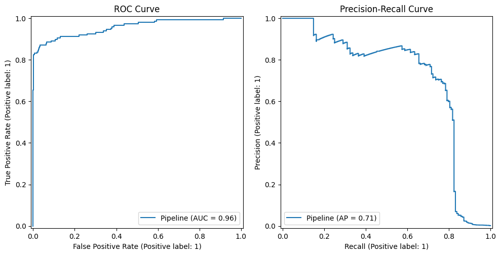
An instance ROC curve and precision-recall curve
Picture by Creator
As an example the use and comparability between ROC AUC and precision-recall (PR curve for brief), we are going to think about three datasets with completely different ranges of sophistication imbalance: from mildly to extremely imbalanced. First, we are going to import every thing we want for all three examples:
|
import pandas as pd from sklearn.datasets import load_breast_cancer from sklearn.model_selection import train_test_split from sklearn.linear_model import LogisticRegression from sklearn.preprocessing import StandardScaler from sklearn.pipeline import make_pipeline from sklearn.metrics import roc_auc_score, average_precision_score |
Instance 1: Gentle Imbalance and Completely different Efficiency Amongst Curves
The Pima Indians Diabetes Dataset is barely imbalanced: about 35% of sufferers are identified with diabetes (class label equals 1), and the opposite 65% have a unfavorable diabetes prognosis (class label equals 0).
This code masses the info, prepares it, trains a binary classifier primarily based on logistic regression, and calculates the world below the 2 varieties of curves being mentioned:
|
1 2 3 4 5 6 7 8 9 10 11 12 13 14 15 16 17 18 19 20 21 |
# Get the info cols = [“preg”,“glucose”,“bp”,“skin”,“insulin”,“bmi”,“pedigree”,“age”,“class”] df = pd.read_csv(“https://uncooked.githubusercontent.com/jbrownlee/Datasets/grasp/pima-indians-diabetes.knowledge.csv”, names=cols)
# Separate labels and cut up into training-test X, y = df.drop(“class”, axis=1), df[“class”] X_train, X_test, y_train, y_test = train_test_split( X, y, stratify=y, test_size=0.3, random_state=42 )
# Scale knowledge and practice classifier clf = make_pipeline( StandardScaler(), LogisticRegression(max_iter=1000) ).match(X_train, y_train)
# Acquire ROC AUC and precision-recall AUC probs = clf.predict_proba(X_test)[:,1] print(“ROC AUC:”, roc_auc_score(y_test, probs)) print(“PR AUC:”, average_precision_score(y_test, probs)) |
On this case, we received a ROC-AUC roughly equal to 0.838, and a PR-AUC of 0.733. As we will observe, the PR AUC (precision-recall) is reasonably decrease than the ROC AUC, which is a typical sample in lots of datasets as a result of ROC AUC tends to overestimate classification efficiency on imbalanced datasets. The next instance makes use of a equally imbalanced dataset with completely different outcomes.
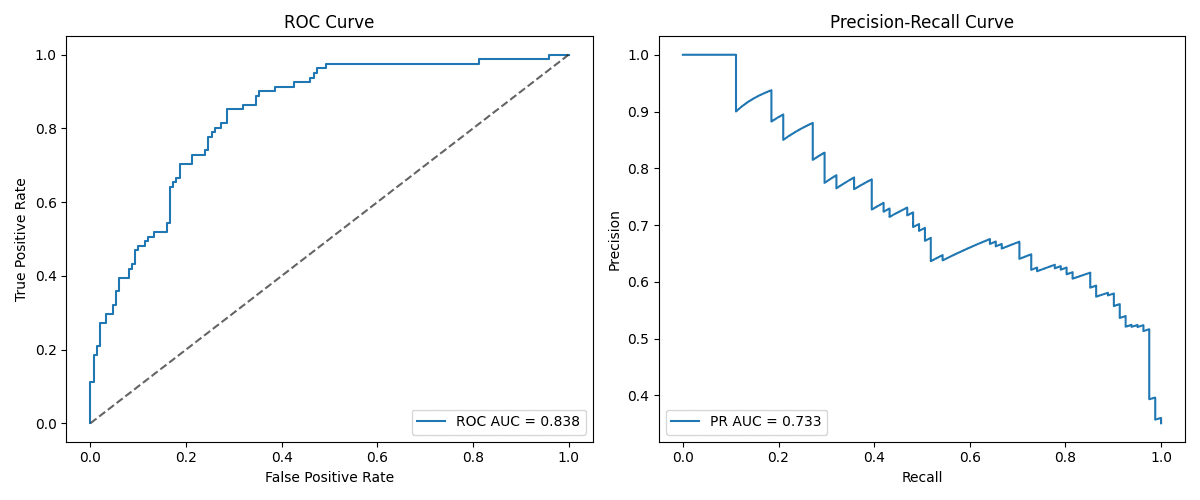
Picture by Editor
Instance 2: Gentle Imbalance and Comparable Efficiency Amongst Curves
One other imbalanced dataset with fairly comparable class proportions to the earlier ones is the Wisconsin Breast Most cancers dataset out there at scikit-learn, with 37% of situations being optimistic.
We apply an analogous course of to the earlier instance within the new dataset and analyze the outcomes.
|
knowledge = load_breast_cancer() X, y = knowledge.knowledge, (knowledge.goal==1).astype(int)
X_train, X_test, y_train, y_test = train_test_split( X, y, stratify=y, test_size=0.3, random_state=42 )
clf = make_pipeline( StandardScaler(), LogisticRegression(max_iter=1000) ).match(X_train, y_train)
probs = clf.predict_proba(X_test)[:,1] print(“ROC AUC:”, roc_auc_score(y_test, probs)) print(“PR AUC:”, average_precision_score(y_test, probs)) |
On this case, we get an ROC AUC of 0.9981016355140186 and a PR AUC of 0.9988072626510498. That is an instance that demonstrates that metric-specific mannequin efficiency usually is dependent upon a lot of components mixed, and never solely class imbalance. Whereas class imbalance usually could replicate a distinction between PR vs ROC AUC, dataset traits like the scale, complexity, sign power from attributes, and so on., are additionally influential. This specific dataset yielded a fairly well-performing classifier total, which can partly clarify its robustness to class imbalance (given the excessive PR AUC obtained).
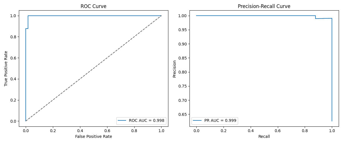
Picture by Editor
Instance 3: Excessive Imbalance
The final instance makes use of a extremely imbalanced dataset, particularly, the bank card fraud detection dataset, wherein lower than 1% of its almost 285K situations belong to the optimistic class, indicating a transaction labeled as fraud.
|
1 2 3 4 5 6 7 8 9 10 11 12 13 14 15 16 17 |
url = ‘https://uncooked.githubusercontent.com/nsethi31/Kaggle-Knowledge-Credit score-Card-Fraud-Detection/grasp/creditcard.csv’ df = pd.read_csv(url)
X, y = df.drop(“Class”, axis=1), df[“Class”]
X_train, X_test, y_train, y_test = train_test_split( X, y, stratify=y, test_size=0.3, random_state=42 )
clf = make_pipeline( StandardScaler(), LogisticRegression(max_iter=2000) ).match(X_train, y_train)
probs = clf.predict_proba(X_test)[:,1] print(“ROC AUC:”, roc_auc_score(y_test, probs)) print(“PR AUC:”, average_precision_score(y_test, probs)) |
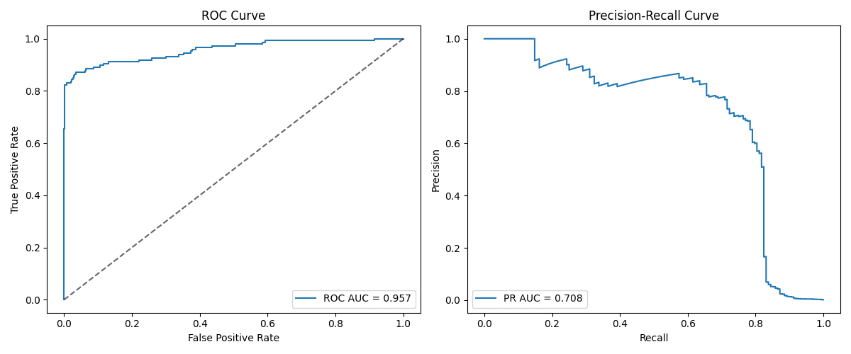
This instance clearly exhibits what usually happens with extremely imbalanced datasets: with an obtained ROC AUC of 0.957 and a PR AUC of 0.708, now we have a robust overestimation of the mannequin efficiency in line with the ROC curve. Which means that whereas ROC seems very promising, the truth is that optimistic circumstances should not being correctly captured, because of being uncommon. A frequent sample is that the stronger the imbalance, the larger the distinction between ROC AUC and PR AUC tends to be.
Picture by Editor
Wrapping Up
This text mentioned and in contrast two widespread metrics to judge classifier efficiency: ROC and precision-recall curves. By three examples on imbalanced datasets, we confirmed the habits and beneficial makes use of of those metrics in numerous eventualities, with the overall key lesson being that precision-recall curves are typically a extra informative and real looking solution to consider classifiers for class-imbalanced knowledge.
For additional studying on find out how to navigate imbalanced datasets for classification, try this text.
ROC AUC vs Precision-Recall for Imbalanced Knowledge
Picture by Editor | ChatGPT
Introduction
When constructing machine studying fashions to categorise imbalanced knowledge — i.e. datasets the place the presence of 1 class (like spam e-mail for instance) is far much less frequent than the presence of the opposite class (non-spam e-mail, as an illustration) — sure conventional metrics like accuracy and even the ROC AUC (Receiving Working Attribute curve and the world below it) could not replicate the mannequin efficiency in real looking phrases, giving overly optimistic estimates because of the dominance of the so-called unfavorable class.
Precision-recall curves (or PR curves for brief), alternatively, are designed to focus particularly on the optimistic, usually rarer class, which is a way more informative measure for skewed datasets because of class imbalance.
By a dialogue and three sensible instance eventualities, this text gives a comparability between ROC AUC and PR AUC — the world below each curves, taking values between 0 and 1 — throughout three imbalanced datasets, by coaching and evaluating a easy classifier primarily based on logistic regression.
ROC AUC vs Precision-Recall
The ROC curve is the go-to method to judge a classifier’s means to discriminate between courses, particularly by plotting the TPR (True Constructive Charge, additionally known as recall) towards the FPR (False Constructive Charge) for various thresholds for the likelihood of belonging to the optimistic class. In the meantime, the precision-recall (PR) curve plots precision towards recall for various thresholds, specializing in analyzing efficiency for optimistic class predictions. Due to this fact, it’s notably helpful and informative for comprehensively evaluating classifiers skilled on imbalanced datasets. The ROC curve, alternatively, is much less delicate to class imbalance, being extra appropriate for evaluating classifiers constructed on fairly balanced datasets, in addition to in eventualities the place the real-world value of false optimistic and false unfavorable predictions is analogous.
In sum, again to the PR curve and sophistication imbalance datasets, in high-stakes eventualities the place accurately figuring out positive-class situations is essential (e.g. figuring out the presence of a illness in a affected person), the PR curve is a extra dependable measure of the classifier’s efficiency.
On a extra visible observe, if we plot each curves alongside one another, we must always get an rising curve within the case of ROC and a lowering curve within the case of PR. The nearer the ROC curve will get to the (0,1) level, which means the best TPR and the bottom FPR, the higher; whereas the nearer the PR curve will get to the (1,1) level, which means each precision and recall are at their most, the higher. In each bases, getting nearer to those “excellent mannequin factors” means the world below the curve or AUC turns into most: that is the numerical worth we are going to search within the examples that comply with.
An instance ROC curve and precision-recall curve
Picture by Creator
As an example the use and comparability between ROC AUC and precision-recall (PR curve for brief), we are going to think about three datasets with completely different ranges of sophistication imbalance: from mildly to extremely imbalanced. First, we are going to import every thing we want for all three examples:
|
import pandas as pd from sklearn.datasets import load_breast_cancer from sklearn.model_selection import train_test_split from sklearn.linear_model import LogisticRegression from sklearn.preprocessing import StandardScaler from sklearn.pipeline import make_pipeline from sklearn.metrics import roc_auc_score, average_precision_score |
Instance 1: Gentle Imbalance and Completely different Efficiency Amongst Curves
The Pima Indians Diabetes Dataset is barely imbalanced: about 35% of sufferers are identified with diabetes (class label equals 1), and the opposite 65% have a unfavorable diabetes prognosis (class label equals 0).
This code masses the info, prepares it, trains a binary classifier primarily based on logistic regression, and calculates the world below the 2 varieties of curves being mentioned:
|
1 2 3 4 5 6 7 8 9 10 11 12 13 14 15 16 17 18 19 20 21 |
# Get the info cols = [“preg”,“glucose”,“bp”,“skin”,“insulin”,“bmi”,“pedigree”,“age”,“class”] df = pd.read_csv(“https://uncooked.githubusercontent.com/jbrownlee/Datasets/grasp/pima-indians-diabetes.knowledge.csv”, names=cols)
# Separate labels and cut up into training-test X, y = df.drop(“class”, axis=1), df[“class”] X_train, X_test, y_train, y_test = train_test_split( X, y, stratify=y, test_size=0.3, random_state=42 )
# Scale knowledge and practice classifier clf = make_pipeline( StandardScaler(), LogisticRegression(max_iter=1000) ).match(X_train, y_train)
# Acquire ROC AUC and precision-recall AUC probs = clf.predict_proba(X_test)[:,1] print(“ROC AUC:”, roc_auc_score(y_test, probs)) print(“PR AUC:”, average_precision_score(y_test, probs)) |
On this case, we received a ROC-AUC roughly equal to 0.838, and a PR-AUC of 0.733. As we will observe, the PR AUC (precision-recall) is reasonably decrease than the ROC AUC, which is a typical sample in lots of datasets as a result of ROC AUC tends to overestimate classification efficiency on imbalanced datasets. The next instance makes use of a equally imbalanced dataset with completely different outcomes.
Picture by Editor
Instance 2: Gentle Imbalance and Comparable Efficiency Amongst Curves
One other imbalanced dataset with fairly comparable class proportions to the earlier ones is the Wisconsin Breast Most cancers dataset out there at scikit-learn, with 37% of situations being optimistic.
We apply an analogous course of to the earlier instance within the new dataset and analyze the outcomes.
|
knowledge = load_breast_cancer() X, y = knowledge.knowledge, (knowledge.goal==1).astype(int)
X_train, X_test, y_train, y_test = train_test_split( X, y, stratify=y, test_size=0.3, random_state=42 )
clf = make_pipeline( StandardScaler(), LogisticRegression(max_iter=1000) ).match(X_train, y_train)
probs = clf.predict_proba(X_test)[:,1] print(“ROC AUC:”, roc_auc_score(y_test, probs)) print(“PR AUC:”, average_precision_score(y_test, probs)) |
On this case, we get an ROC AUC of 0.9981016355140186 and a PR AUC of 0.9988072626510498. That is an instance that demonstrates that metric-specific mannequin efficiency usually is dependent upon a lot of components mixed, and never solely class imbalance. Whereas class imbalance usually could replicate a distinction between PR vs ROC AUC, dataset traits like the scale, complexity, sign power from attributes, and so on., are additionally influential. This specific dataset yielded a fairly well-performing classifier total, which can partly clarify its robustness to class imbalance (given the excessive PR AUC obtained).
Picture by Editor
Instance 3: Excessive Imbalance
The final instance makes use of a extremely imbalanced dataset, particularly, the bank card fraud detection dataset, wherein lower than 1% of its almost 285K situations belong to the optimistic class, indicating a transaction labeled as fraud.
|
1 2 3 4 5 6 7 8 9 10 11 12 13 14 15 16 17 |
url = ‘https://uncooked.githubusercontent.com/nsethi31/Kaggle-Knowledge-Credit score-Card-Fraud-Detection/grasp/creditcard.csv’ df = pd.read_csv(url)
X, y = df.drop(“Class”, axis=1), df[“Class”]
X_train, X_test, y_train, y_test = train_test_split( X, y, stratify=y, test_size=0.3, random_state=42 )
clf = make_pipeline( StandardScaler(), LogisticRegression(max_iter=2000) ).match(X_train, y_train)
probs = clf.predict_proba(X_test)[:,1] print(“ROC AUC:”, roc_auc_score(y_test, probs)) print(“PR AUC:”, average_precision_score(y_test, probs)) |
This instance clearly exhibits what usually happens with extremely imbalanced datasets: with an obtained ROC AUC of 0.957 and a PR AUC of 0.708, now we have a robust overestimation of the mannequin efficiency in line with the ROC curve. Which means that whereas ROC seems very promising, the truth is that optimistic circumstances should not being correctly captured, because of being uncommon. A frequent sample is that the stronger the imbalance, the larger the distinction between ROC AUC and PR AUC tends to be.
Picture by Editor
Wrapping Up
This text mentioned and in contrast two widespread metrics to judge classifier efficiency: ROC and precision-recall curves. By three examples on imbalanced datasets, we confirmed the habits and beneficial makes use of of those metrics in numerous eventualities, with the overall key lesson being that precision-recall curves are typically a extra informative and real looking solution to consider classifiers for class-imbalanced knowledge.
For additional studying on find out how to navigate imbalanced datasets for classification, try this text.


