


Picture by Editor | Midjourney
Whereas Python-based instruments like Streamlit are common for creating knowledge dashboards, Excel stays one of the crucial accessible and highly effective platforms for constructing interactive knowledge visualizations. Utilizing built-in Excel’s options, you may construct an interactive dashboard that rivals common knowledge science internet apps.
On this tutorial, we are going to present the right way to create an interactive knowledge science dashboard in Excel in minutes with out Streamlit. We are going to reveal utilizing a easy e-commerce gross sales dataset.
Step 1: Making ready Your Dataset
We are going to break up this step up into subcomponents and deal with every one after the other.
Set Up Your Information
To arrange the Excel workbook we will probably be utilizing, comply with these steps:
- Open a brand new Excel workbook
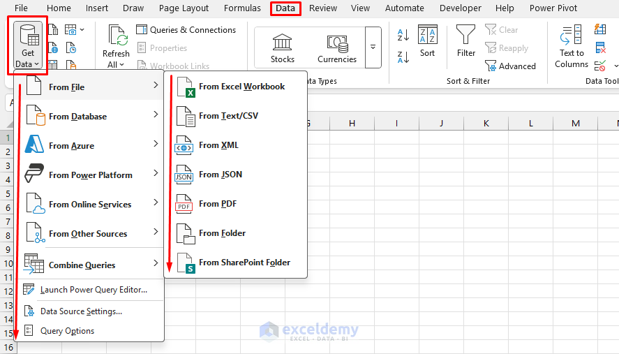
- Import your knowledge into Excel
- Go to the Information tab >> choose Get Information >> choose your file kind
- Carry out any dataset cleansing or upkeep which may be required
Convert to Excel Desk
Subsequent, let’s convert our knowledge to an Excel desk. Tables make it simple to construct formulation, PivotTables, and dynamic ranges.
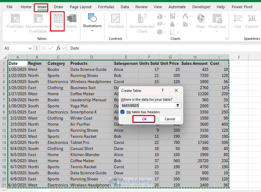
- Choose your complete dataset
- Go to the Insert tab >> choose Desk (or press Ctrl+T)
- Guarantee My desk has headers is checked
- Click on OK
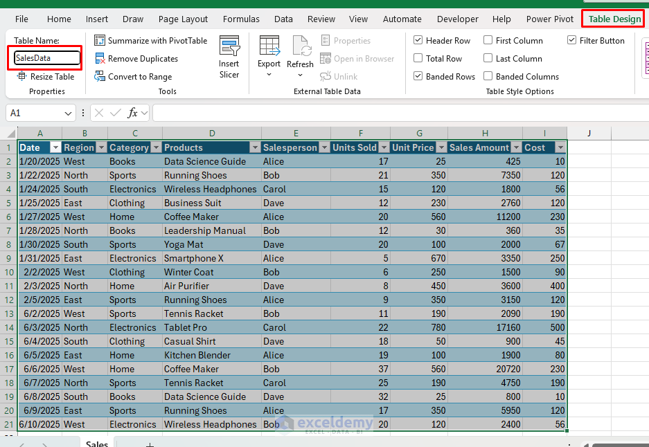
- Identify your desk SalesData:
- Click on wherever within the desk
- Go to the Desk Design tab >> choose Desk Identify >> kind SalesData
Step 2: Create Interactive Pivot Tables
Create Pivot Desk:
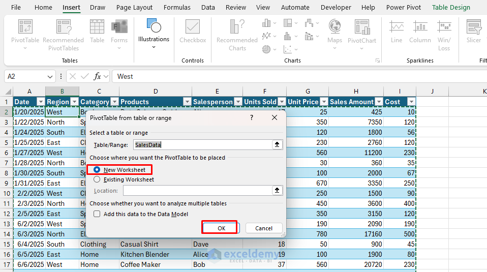
- Choose any cell within the SalesData desk.
- Go to the Insert tab >> choose PivotTable.
- Choose location: New Worksheet.
- Click on OK.
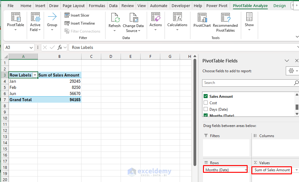
Income by Month:
- Within the PivotTable FieldList:
- Rows: Date (group by Months).
- Values: Gross sales Quantity.
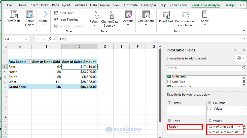
Regional Efficiency:
- Insert one other PivotTable.
- Within the PivotTable FieldList:
- Rows: Area.
- Values: Gross sales Quantity, Models Offered.
- Format: Forex for Gross sales Quantity.
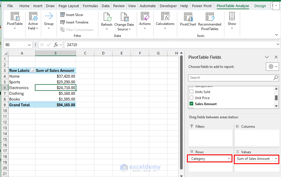
Product Class Evaluation:
- Insert one other PivotTable.
- Within the PivotTable FieldList:
- Rows: Class.
- Values: Gross sales Quantity.
- Type: Descending by Gross sales Quantity.
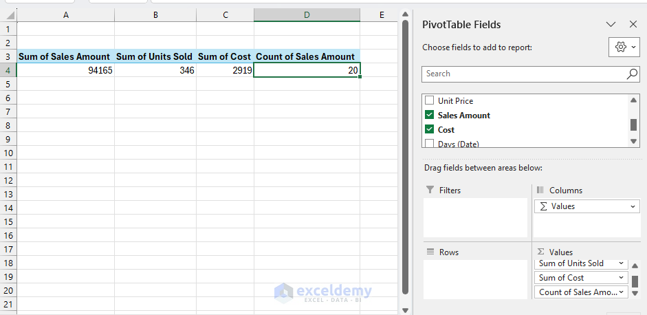
KPIs Pivot Desk:
- Insert one other PivotTable.
- Within the PivotTable FieldList:
- Values:
- Sum of Gross sales Quantity.
- Sum of Models Offered.
- Sum of Price.
- Rely of Gross sales Quantity (for common calculation).
- Do not add any Rows or Columns (this provides us totals).
Step 3: Create Dynamic Charts
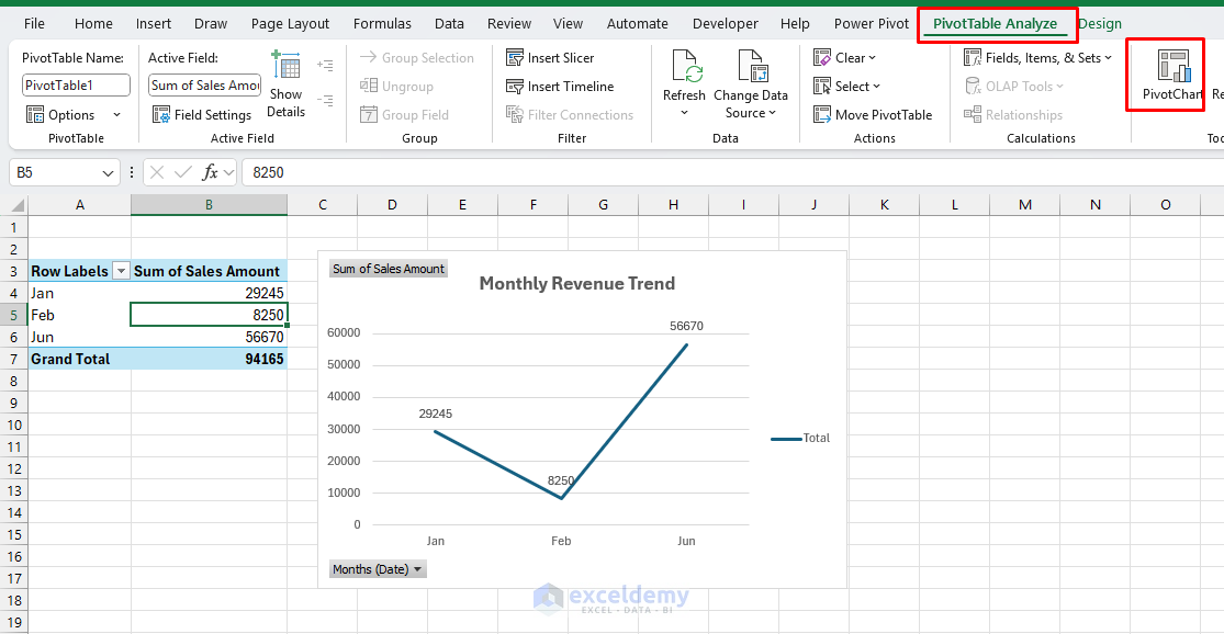
Income Development Line Chart:
- Choose the Month-to-month Income pivot desk.
- Go to the PivotTable Analyze tab >> choose Pivot Chart >> choose Line Chart.
- Format the chart:
- Chart Title: Month-to-month Income Development.
- Add knowledge labels: Increase Chart Parts >> click on Information Labels.
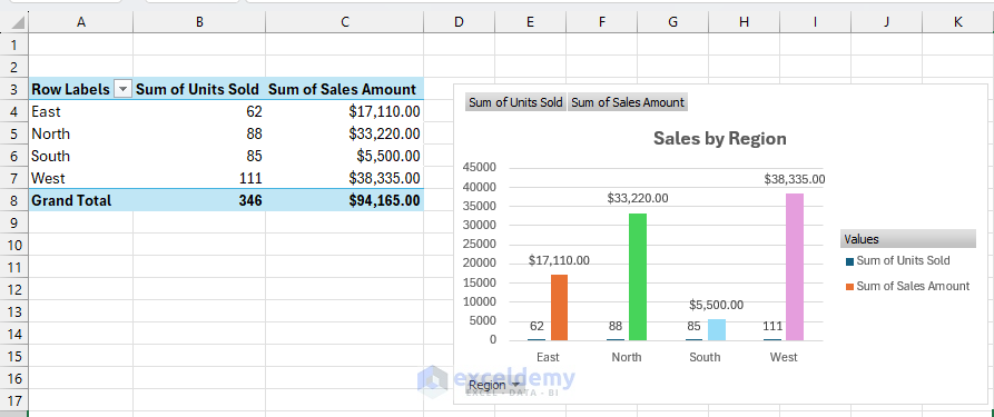
Regional Efficiency Column Chart
- Choose the Regional pivot desk.
- Go to the PivotTable Analyze tab >> choose Pivot Chart >> choose Clustered Column.
- Format:
- Title: Gross sales by Area.
- Totally different colours for every area.
- Information labels on prime of columns.
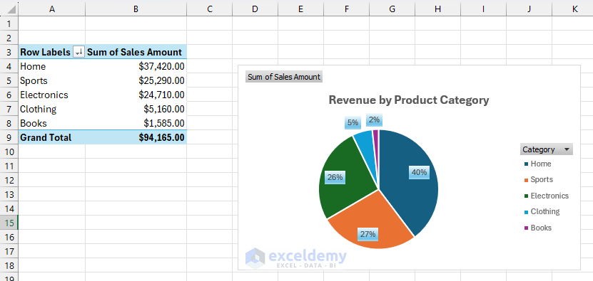
Product Class Pie Chart
- Choose the Product Class pivot desk.
- Go to the PivotTable Analyze tab >> choose Pivot Chart >> choose Pie Chart.
- Format:
- Title: Income by Product Class.
- Present percentages.
- Use distinct colours.
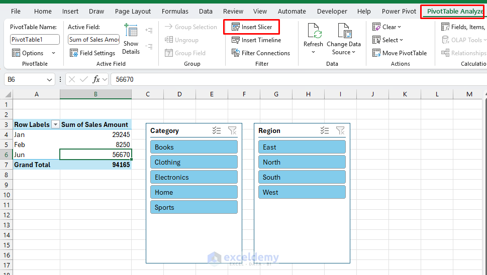
Step 4: Add Interactive Slicers
Insert Slicers:
- Click on on any pivot desk.
- Go to the PivotTable Analyze tab >> choose Insert Slicer.
- Choose these fields:
- Click on OK.
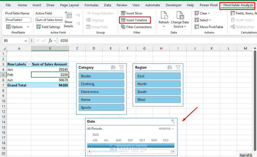
Insert Timeline:
- Click on on any pivot desk.
- Go to the PivotTable Analyze tab >> choose Insert Timeline.
- Choose Date.
- Click on OK.
Join Slicers to All Pivot Tables:
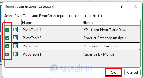
- Proper-click any slicer >> choose Report Connections.
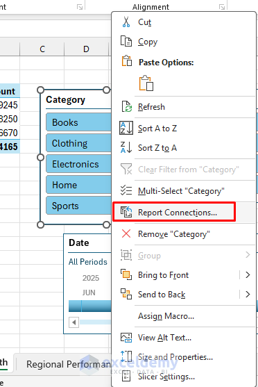
- Examine all pivot tables.
- Click on OK.
Repeat for every slicer to make sure all of them management all charts.
Step 5: Construct Dynamic KPI Playing cards
You’ll be able to calculate KPI metrics instantly within the Dashboard or later place it within the Dashboard sheet.
Now create KPIs that reference this pivot desk:
Whole Gross sales:
- Choose a cell and insert the next formulation.
=GETPIVOTDATA("Sum of Gross sales Quantity",'KPIs from Pivot Desk Information'!$A$3)
Common Order Worth:
- Choose a cell and insert the next formulation.
=GETPIVOTDATA("Sum of Gross sales Quantity",'KPIs from Pivot Desk Information'!$A$3)/GETPIVOTDATA("Rely of Gross sales Quantity",'KPIs from Pivot Desk Information'!$A$3)
Whole Models Offered:
- Choose a cell and insert the next formulation.
=GETPIVOTDATA("Sum of Models Offered",'KPIs from Pivot Desk Information'!$A$3)
Revenue Margin %:
- Choose a cell and insert the next formulation.
=(GETPIVOTDATA("Sum of Gross sales Quantity",'KPIs from Pivot Desk Information'!$A$3)-GETPIVOTDATA("Sum of Price",'KPIs from Pivot Desk Information'!$A$3))/GETPIVOTDATA("Sum of Gross sales Quantity",'KPIs from Pivot Desk Information'!$A$3)
Whole Order:
- Choose a cell and insert the next formulation.
=GETPIVOTDATA("Rely of Gross sales Quantity",'KPIs from Pivot Desk Information'!$A$3)
Format KPI Playing cards:
- Apply borders and alignment.
- Format numbers:
- Income: Forex format.
- Share: Share format with 2 decimals.
- Daring the labels and add background shade.
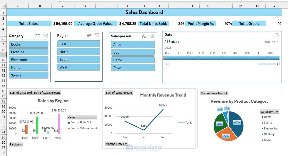
Step 6: Create the Dashboard Construction
- Create a brand new sheet and identify it Dashboard.
- Cover Gridlines:
- Go to the View tab >> choose Present >> uncheck Gridlines.
- Insert Dashboard title.
- Place KPI metrics on the prime.
- Insert Slicers and a timeline.
- Place charts on the backside.
- Insert a knowledge desk if required.
Refresh and Automate: Proper-click PivotTables/Charts >> choose Refresh.
Step 7: Take a look at Your Dashboard
Performance Exams:
- Choose Books class + North area + Bob salesperson from Slicers.
- Choose Jan 2025 from Timeline.
- Confirm that each one charts replace concurrently.
- Examine that KPIs are recalculated appropriately.
- Guarantee no errors seem.

Troubleshoot Frequent Points
- Charts Not Updating: Examine slicer connections (right-click slicer > Report Connections). Guarantee all pivot tables are chosen.
- Method Errors: #REF! or #VALUE! errors in KPIs. Examine desk references (guarantee SalesData desk identify is appropriate).
- Efficiency Points: Dashboard is gradual to replace:
- Cut back the variety of pivot tables.
- Simplify complicated formulation.
- Use handbook calculation (Formulation > Calculation Choices > Handbook).
Conclusion
By following the above steps, you may create an interactive knowledge science dashboard in Excel in minutes. These steps will enable you to create refined dashboards that present actual enterprise worth with out touching a single line of Python code. The most effective half is that your stakeholders can work together with and modify the dashboard themselves, making it a really collaborative enterprise intelligence software.
Shamima Sultana works as a Undertaking Supervisor at ExcelDemy, the place she does analysis on Microsoft Excel and writes articles associated to her work. Shamima holds a BSc in Pc Science and Engineering and has an excellent curiosity in analysis and improvement. Shamima likes to study new issues, and is attempting to offer enriched high quality content material concerning Excel, whereas all the time attempting to assemble information from varied sources and making revolutionary options.
Picture by Editor | Midjourney
Whereas Python-based instruments like Streamlit are common for creating knowledge dashboards, Excel stays one of the crucial accessible and highly effective platforms for constructing interactive knowledge visualizations. Utilizing built-in Excel’s options, you may construct an interactive dashboard that rivals common knowledge science internet apps.
On this tutorial, we are going to present the right way to create an interactive knowledge science dashboard in Excel in minutes with out Streamlit. We are going to reveal utilizing a easy e-commerce gross sales dataset.
Step 1: Making ready Your Dataset
We are going to break up this step up into subcomponents and deal with every one after the other.
Set Up Your Information
To arrange the Excel workbook we will probably be utilizing, comply with these steps:
- Open a brand new Excel workbook
- Import your knowledge into Excel
- Go to the Information tab >> choose Get Information >> choose your file kind
- Carry out any dataset cleansing or upkeep which may be required
Convert to Excel Desk
Subsequent, let’s convert our knowledge to an Excel desk. Tables make it simple to construct formulation, PivotTables, and dynamic ranges.
- Choose your complete dataset
- Go to the Insert tab >> choose Desk (or press Ctrl+T)
- Guarantee My desk has headers is checked
- Click on OK
- Identify your desk SalesData:
- Click on wherever within the desk
- Go to the Desk Design tab >> choose Desk Identify >> kind SalesData
Step 2: Create Interactive Pivot Tables
Create Pivot Desk:
- Choose any cell within the SalesData desk.
- Go to the Insert tab >> choose PivotTable.
- Choose location: New Worksheet.
- Click on OK.
Income by Month:
- Within the PivotTable FieldList:
- Rows: Date (group by Months).
- Values: Gross sales Quantity.
Regional Efficiency:
- Insert one other PivotTable.
- Within the PivotTable FieldList:
- Rows: Area.
- Values: Gross sales Quantity, Models Offered.
- Format: Forex for Gross sales Quantity.
Product Class Evaluation:
- Insert one other PivotTable.
- Within the PivotTable FieldList:
- Rows: Class.
- Values: Gross sales Quantity.
- Type: Descending by Gross sales Quantity.
KPIs Pivot Desk:
- Insert one other PivotTable.
- Within the PivotTable FieldList:
- Values:
- Sum of Gross sales Quantity.
- Sum of Models Offered.
- Sum of Price.
- Rely of Gross sales Quantity (for common calculation).
- Do not add any Rows or Columns (this provides us totals).
Step 3: Create Dynamic Charts
Income Development Line Chart:
- Choose the Month-to-month Income pivot desk.
- Go to the PivotTable Analyze tab >> choose Pivot Chart >> choose Line Chart.
- Format the chart:
- Chart Title: Month-to-month Income Development.
- Add knowledge labels: Increase Chart Parts >> click on Information Labels.
Regional Efficiency Column Chart
- Choose the Regional pivot desk.
- Go to the PivotTable Analyze tab >> choose Pivot Chart >> choose Clustered Column.
- Format:
- Title: Gross sales by Area.
- Totally different colours for every area.
- Information labels on prime of columns.
Product Class Pie Chart
- Choose the Product Class pivot desk.
- Go to the PivotTable Analyze tab >> choose Pivot Chart >> choose Pie Chart.
- Format:
- Title: Income by Product Class.
- Present percentages.
- Use distinct colours.
Step 4: Add Interactive Slicers
Insert Slicers:
- Click on on any pivot desk.
- Go to the PivotTable Analyze tab >> choose Insert Slicer.
- Choose these fields:
- Click on OK.
Insert Timeline:
- Click on on any pivot desk.
- Go to the PivotTable Analyze tab >> choose Insert Timeline.
- Choose Date.
- Click on OK.
Join Slicers to All Pivot Tables:
- Proper-click any slicer >> choose Report Connections.
- Examine all pivot tables.
- Click on OK.
Repeat for every slicer to make sure all of them management all charts.
Step 5: Construct Dynamic KPI Playing cards
You’ll be able to calculate KPI metrics instantly within the Dashboard or later place it within the Dashboard sheet.
Now create KPIs that reference this pivot desk:
Whole Gross sales:
- Choose a cell and insert the next formulation.
=GETPIVOTDATA("Sum of Gross sales Quantity",'KPIs from Pivot Desk Information'!$A$3)
Common Order Worth:
- Choose a cell and insert the next formulation.
=GETPIVOTDATA("Sum of Gross sales Quantity",'KPIs from Pivot Desk Information'!$A$3)/GETPIVOTDATA("Rely of Gross sales Quantity",'KPIs from Pivot Desk Information'!$A$3)
Whole Models Offered:
- Choose a cell and insert the next formulation.
=GETPIVOTDATA("Sum of Models Offered",'KPIs from Pivot Desk Information'!$A$3)
Revenue Margin %:
- Choose a cell and insert the next formulation.
=(GETPIVOTDATA("Sum of Gross sales Quantity",'KPIs from Pivot Desk Information'!$A$3)-GETPIVOTDATA("Sum of Price",'KPIs from Pivot Desk Information'!$A$3))/GETPIVOTDATA("Sum of Gross sales Quantity",'KPIs from Pivot Desk Information'!$A$3)
Whole Order:
- Choose a cell and insert the next formulation.
=GETPIVOTDATA("Rely of Gross sales Quantity",'KPIs from Pivot Desk Information'!$A$3)
Format KPI Playing cards:
- Apply borders and alignment.
- Format numbers:
- Income: Forex format.
- Share: Share format with 2 decimals.
- Daring the labels and add background shade.
Step 6: Create the Dashboard Construction
- Create a brand new sheet and identify it Dashboard.
- Cover Gridlines:
- Go to the View tab >> choose Present >> uncheck Gridlines.
- Insert Dashboard title.
- Place KPI metrics on the prime.
- Insert Slicers and a timeline.
- Place charts on the backside.
- Insert a knowledge desk if required.
Refresh and Automate: Proper-click PivotTables/Charts >> choose Refresh.
Step 7: Take a look at Your Dashboard
Performance Exams:
- Choose Books class + North area + Bob salesperson from Slicers.
- Choose Jan 2025 from Timeline.
- Confirm that each one charts replace concurrently.
- Examine that KPIs are recalculated appropriately.
- Guarantee no errors seem.
Troubleshoot Frequent Points
- Charts Not Updating: Examine slicer connections (right-click slicer > Report Connections). Guarantee all pivot tables are chosen.
- Method Errors: #REF! or #VALUE! errors in KPIs. Examine desk references (guarantee SalesData desk identify is appropriate).
- Efficiency Points: Dashboard is gradual to replace:
- Cut back the variety of pivot tables.
- Simplify complicated formulation.
- Use handbook calculation (Formulation > Calculation Choices > Handbook).
Conclusion
By following the above steps, you may create an interactive knowledge science dashboard in Excel in minutes. These steps will enable you to create refined dashboards that present actual enterprise worth with out touching a single line of Python code. The most effective half is that your stakeholders can work together with and modify the dashboard themselves, making it a really collaborative enterprise intelligence software.
Shamima Sultana works as a Undertaking Supervisor at ExcelDemy, the place she does analysis on Microsoft Excel and writes articles associated to her work. Shamima holds a BSc in Pc Science and Engineering and has an excellent curiosity in analysis and improvement. Shamima likes to study new issues, and is attempting to offer enriched high quality content material concerning Excel, whereas all the time attempting to assemble information from varied sources and making revolutionary options.


