


On this article, you’ll learn the way Bag-of-Phrases, TF-IDF, and LLM-generated embeddings evaluate when used as textual content options for classification and clustering in scikit-learn.
Subjects we are going to cowl embody:
- Easy methods to generate Bag-of-Phrases, TF-IDF, and LLM embeddings for a similar dataset.
- How these representations evaluate on textual content classification efficiency and coaching pace.
- How they behave otherwise for unsupervised doc clustering.
Let’s get proper to it.
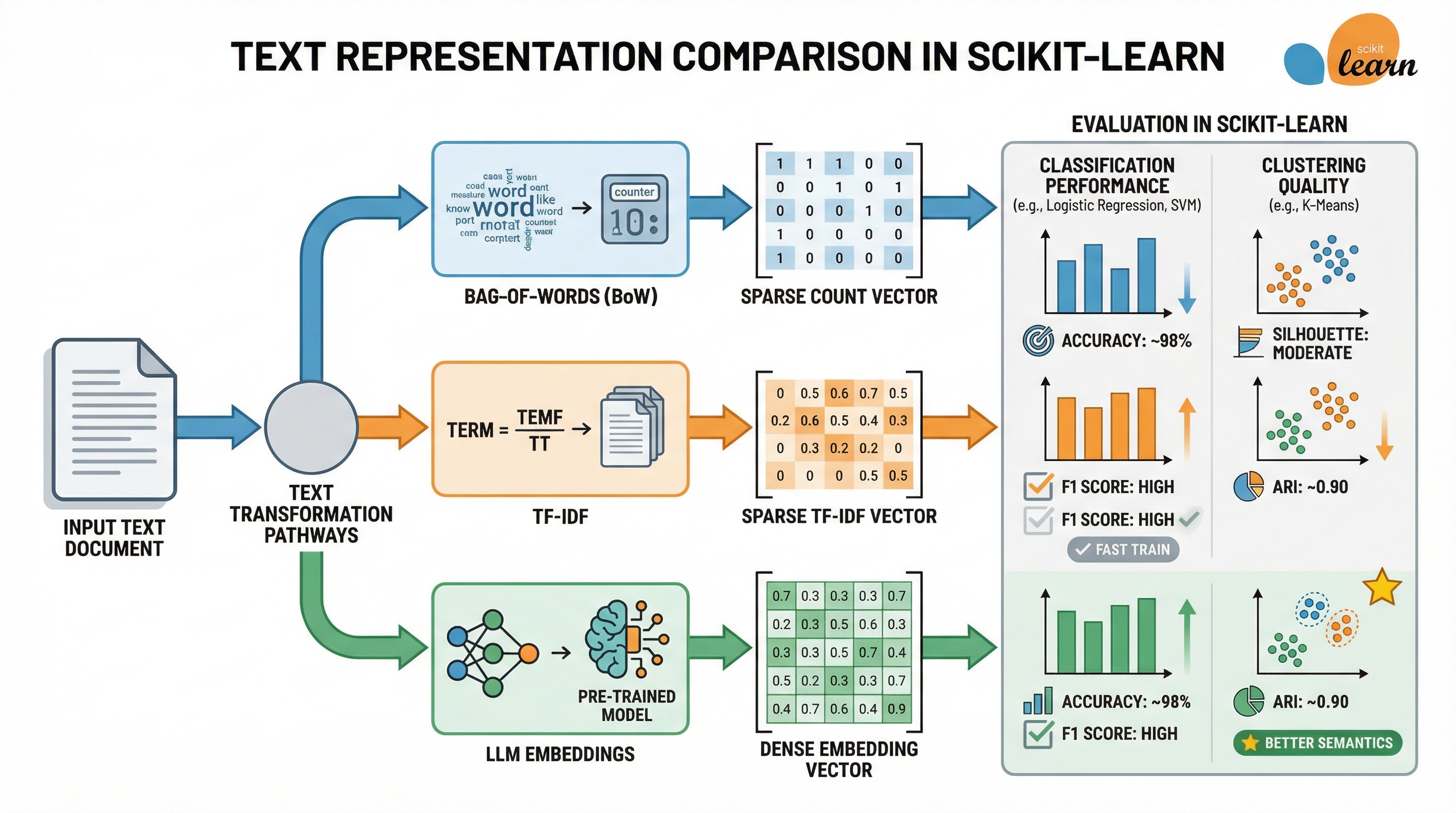
LLM Embeddings vs TF-IDF vs Bag-of-Phrases: Which Works Higher in Scikit-learn? (click on to enlarge)
Picture by Creator
Introduction
Machine studying fashions constructed with frameworks like scikit-learn can accommodate unstructured knowledge like textual content, so long as this uncooked textual content is transformed right into a numerical illustration that’s comprehensible by algorithms, fashions, and machines in a broader sense.
This text takes three well-known textual content illustration approaches — TF-IDF, Bag-of-Phrases, and LLM-generated embeddings — to supply an analytical and example-based comparability between them, within the context of downstream machine studying modeling with scikit-learn.
For a glimpse of textual content illustration approaches, together with an introduction to the three used on this article, we advocate you check out this text and this one.
The article will first navigate you thru a Python instance the place we are going to use the BBC information dataset — a labeled dataset containing a couple of thousand information articles categorized into 5 varieties — to acquire the three goal representations for every textual content, construct some textual content classifiers and evaluate them, and in addition construct and evaluate some clustering fashions. After that, we undertake a extra basic and analytical perspective to debate which method is best — and when to make use of one or one other.
Setup and Getting Textual content Representations
First, we import all of the modules and libraries we are going to want, arrange some configurations, and cargo the BBC information dataset:
|
1 2 3 4 5 6 7 8 9 10 11 12 13 14 15 16 17 18 19 20 21 22 23 24 25 26 27 28 29 30 31 32 33 34 35 |
import pandas as pd import numpy as np import matplotlib.pyplot as plt import seaborn as sns from time import time
# Scikit-learn imports from sklearn.feature_extraction.textual content import CountVectorizer, TfidfVectorizer from sklearn.model_selection import train_test_split, cross_val_score from sklearn.linear_model import LogisticRegression from sklearn.ensemble import RandomForestClassifier from sklearn.svm import SVC from sklearn.cluster import KMeans from sklearn.metrics import ( accuracy_score, f1_score, classification_report, silhouette_score, adjusted_rand_rating ) from sklearn.preprocessing import LabelEncoder
# Our key import for constructing LLM embeddings: a Sentence Transformer mannequin from sentence_transformers import SentenceTransformer
# Plotting configuration – for later analyzing and evaluating outcomes sns.set_style(“whitegrid”) plt.rcParams[‘figure.figsize’] = (14, 6)
# Loading BBC Information dataset print(“Loading BBC Information dataset…”) url = “https://storage.googleapis.com/dataset-uploader/bbc/bbc-text.csv” df = pd.read_csv(url)
print(f“Dataset loaded: {len(df)} paperwork”) print(f“Classes: {df[‘category’].distinctive()}”) print(f“nClass distribution:”) print(df[‘category’].value_counts()) |
On the time of writing, the dataset model we’re utilizing incorporates 2225 situations, that’s, paperwork containing information articles.
Since we are going to prepare some supervised machine studying fashions for classification in a while, earlier than acquiring the three representations for our textual content knowledge, we separate the enter texts from their labels and break up the entire dataset into coaching and take a look at subsets:
|
1 2 3 4 5 6 7 8 9 10 11 12 13 14 15 16 17 |
print(“n” + “=”*70) print(“DATA PREPARATION PRIOR TO GENERATING TEXT REPRESENTATIONS”) print(“=”*70)
texts = df[‘text’].tolist() labels = df[‘category’].tolist()
# Encoding labels for classification le = LabelEncoder() y = le.fit_transform(labels)
# Splitting knowledge (identical break up for all illustration strategies and ML fashions educated later) X_text_train, X_text_test, y_train, y_test = train_test_split( texts, y, test_size=0.2, random_state=42, stratify=y )
print(f“nTrain set: {len(X_text_train)} | Take a look at set: {len(X_text_test)}”) |
Illustration 1: Bag-of-Phrases (BoW)
|
1 2 3 4 5 6 7 8 9 10 11 12 13 14 15 16 17 18 19 |
print(“n[1] Bag-of-Phrases…”) begin = time()
# The CountVectorizer class is used to use BoW bow_vectorizer = CountVectorizer( max_features=5000, min_df=2, stop_words=‘english’ )
X_bow_train = bow_vectorizer.fit_transform(X_text_train) X_bow_test = bow_vectorizer.remodel(X_text_test)
bow_time = time() – begin
print(f” Performed in {bow_time:.2f}s”) print(f” Form: {X_bow_train.form} (paperwork × vocabulary)”) print(f” Sparsity: {(1 – X_bow_train.nnz / (X_bow_train.form[0] * X_bow_train.form[1])) * 100:.1f}%”) print(f” Reminiscence: {X_bow_train.knowledge.nbytes / 1024:.1f} KB”) |
Illustration 2: TF-IDF
|
1 2 3 4 5 6 7 8 9 10 11 12 13 14 15 16 17 18 19 |
print(“n[2] TF-IDF…”) begin = time()
# Utilizing TfidfVectorizer class to use TF-IDF primarily based on phrase frequencies tfidf_vectorizer = TfidfVectorizer( max_features=5000, min_df=2, stop_words=‘english’ )
X_tfidf_train = tfidf_vectorizer.fit_transform(X_text_train) X_tfidf_test = tfidf_vectorizer.remodel(X_text_test)
tfidf_time = time() – begin
print(f” Performed in {tfidf_time:.2f}s”) print(f” Form: {X_tfidf_train.form}”) print(f” Sparsity: {(1 – X_tfidf_train.nnz / (X_tfidf_train.form[0] * X_tfidf_train.form[1])) * 100:.1f}%”) print(f” Reminiscence: {X_tfidf_train.knowledge.nbytes / 1024:.1f} KB”) |
Illustration 3: LLM Embeddings
|
1 2 3 4 5 6 7 8 9 10 11 12 13 14 15 16 17 18 19 20 21 22 23 |
print(“n[3] LLM Embeddings…”) begin = time()
# Loading a pre-trained sentence transformer mannequin to generate 384-dimensional embeddings embedding_model = SentenceTransformer(‘all-MiniLM-L6-v2’)
X_emb_train = embedding_model.encode( X_text_train, show_progress_bar=True, batch_size=32 ) X_emb_test = embedding_model.encode( X_text_test, show_progress_bar=False, batch_size=32 )
emb_time = time() – begin
print(f” Performed in {emb_time:.2f}s”) print(f” Form: {X_emb_train.form} (paperwork × embedding_dim)”) print(f” Sparsity: 0.0% (dense illustration)”) print(f” Reminiscence: {X_emb_train.nbytes / 1024:.1f} KB”) |
Comparability 1: Textual content Classification
That was an intensive preparatory stage! Now we’re prepared for a primary comparability instance, centered on coaching a number of forms of machine studying classifiers and evaluating how every sort of classifier performs when educated on one textual content illustration or one other.
In a nutshell, the code offered under will:
- Take into account three classifier varieties: logistic regression, random forests, and assist vector machines (SVM).
- Practice and consider every of the three×3 = 9 classifiers educated, utilizing two analysis metrics: accuracy and F1 rating.
- Listing and visualize the outcomes obtained from every mannequin sort and textual content illustration method used.
|
1 2 3 4 5 6 7 8 9 10 11 12 13 14 15 16 17 18 19 20 21 22 23 24 25 26 27 28 29 30 31 32 33 34 35 36 37 38 39 40 41 42 43 44 45 46 47 48 49 50 51 52 53 |
print(“n” + “=”*70) print(“COMPARISON 1: SUPERVISED CLASSIFICATION”) print(“=”*70)
# Defining the three forms of classifiers to coach classifiers = { ‘Logistic Regression’: LogisticRegression(max_iter=1000, random_state=42), ‘Random Forest’: RandomForestClassifier(n_estimators=100, random_state=42), ‘SVM’: SVC(kernel=‘linear’, random_state=42) }
# Storing leads to a Python assortment (checklist) classification_results = []
# Evaluating every illustration with every classifier representations = { ‘BoW’: (X_bow_train, X_bow_test), ‘TF-IDF’: (X_tfidf_train, X_tfidf_test), ‘LLM Embeddings’: (X_emb_train, X_emb_test) }
for rep_name, (X_tr, X_te) in representations.gadgets(): print(f“nTesting {rep_name}:”) print(“-“ * 50)
for clf_name, clf in classifiers.gadgets(): # Practice begin = time() clf.match(X_tr, y_train) train_time = time() – begin
# Predict begin = time() y_pred = clf.predict(X_te) pred_time = time() – begin
# Consider acc = accuracy_score(y_test, y_pred) f1 = f1_score(y_test, y_pred, common=‘weighted’)
print(f” {clf_name:20s} | Acc: {acc:.3f} | F1: {f1:.3f} | Practice: {train_time:.2f}s”)
classification_results.append({ ‘Illustration’: rep_name, ‘Classifier’: clf_name, ‘Accuracy’: acc, ‘F1-Rating’: f1, ‘Practice Time’: train_time, ‘Predict Time’: pred_time })
# Changing outcomes to DataFrame for interpretability and simpler comparability results_df = pd.DataFrame(classification_results) |
Output:
|
1 2 3 4 5 6 7 8 9 10 11 12 13 14 15 16 17 18 19 20 21 |
====================================================================== COMPARISON 1: SUPERVISED CLASSIFICATION ======================================================================
Testing BoW: ————————————————————————— Logistic Regression | Acc: 0.982 | F1: 0.982 | Practice: 0.86s Random Forest | Acc: 0.973 | F1: 0.973 | Practice: 2.20s SVM | Acc: 0.984 | F1: 0.984 | Practice: 2.02s
Testing TF–IDF: ————————————————————————— Logistic Regression | Acc: 0.984 | F1: 0.984 | Practice: 0.52s Random Forest | Acc: 0.978 | F1: 0.977 | Practice: 1.79s SVM | Acc: 0.987 | F1: 0.987 | Practice: 2.99s
Testing LLM Embeddings: ————————————————————————— Logistic Regression | Acc: 0.982 | F1: 0.982 | Practice: 0.27s Random Forest | Acc: 0.960 | F1: 0.959 | Practice: 5.21s SVM | Acc: 0.980 | F1: 0.980 | Practice: 0.15s |
Enter code for visualizing outcomes:
|
1 2 3 4 5 6 7 8 9 10 11 12 13 14 15 16 17 18 19 20 21 22 23 24 25 26 27 28 29 30 31 32 33 |
# Creating visualization plots for direct comparability fig, axes = plt.subplots(1, 2, figsize=(16, 6))
# Plot 1: Accuracy comparability pivot_acc = results_df.pivot(index=‘Classifier’, columns=‘Illustration’, values=‘Accuracy’) pivot_acc.plot(sort=‘bar’, ax=axes[0], width=0.8) axes[0].set_title(‘Classification Accuracy by Illustration’, fontsize=14, fontweight=‘daring’) axes[0].set_ylabel(‘Accuracy’) axes[0].set_xlabel(‘Classifier’) axes[0].legend(title=‘Illustration’) axes[0].grid(axis=‘y’, alpha=0.3) axes[0].set_ylim([0.9, 1.0])
# Plot 2: Coaching time comparability pivot_time = results_df.pivot(index=‘Classifier’, columns=‘Illustration’, values=‘Practice Time’) pivot_time.plot(sort=‘bar’, ax=axes[1], width=0.8, colour=[‘#1f77b4’, ‘#ff7f0e’, ‘#2ca02c’]) axes[1].set_title(‘Coaching Time by Illustration’, fontsize=14, fontweight=‘daring’) axes[1].set_ylabel(‘Time (seconds)’) axes[1].set_xlabel(‘Classifier’) axes[1].legend(title=‘Illustration’) axes[1].grid(axis=‘y’, alpha=0.3)
plt.tight_layout() plt.present()
# Figuring out greatest performers print(“nBEST PERFORMERS:”) print(“-“ * 50) best_acc = results_df.loc[results_df[‘Accuracy’].idxmax()] print(f“Greatest Accuracy: {best_acc[‘Representation’]} + {best_acc[‘Classifier’]} = {best_acc[‘Accuracy’]:.3f}”)
quickest = results_df.loc[results_df[‘Train Time’].idxmin()] print(f“Quickest Coaching: {quickest[‘Representation’]} + {quickest[‘Classifier’]} = {quickest[‘Train Time’]:.2f}s”) |
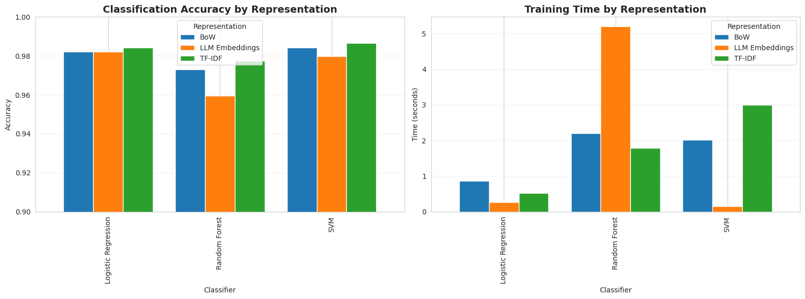
Let’s take these outcomes with a pinch of salt, as they’re particular to the dataset and mannequin varieties educated, and not at all generalizable. TF-IDF mixed with an SVM classifier led to the perfect accuracy (0.987), whereas LLM embeddings with SVM yielded the quickest mannequin to coach (0.15s). In the meantime, the greatest total mixture when it comes to performance-speed steadiness is logistic regression with TF-IDF, with a virtually excellent accuracy of 0.984 and a really quick coaching time of 0.52s.
Why did LLM embeddings, supposedly probably the most superior of the three textual content illustration approaches, not present the perfect efficiency? There are a number of causes for this. First, the present 5 courses (information classes) within the BBC information dataset are strongly word-discriminative; in different phrases, they’re simply separable by class, so reasonably less complicated representations like TF-IDF are sufficient to seize these patterns very nicely. This additionally implies there’s no use for the deep semantic understanding that LLM embeddings obtain; in truth, this will typically be counterproductive and result in overfitting. As well as, due to the close to separability between information varieties, linear and less complicated fashions work nice, in comparison with advanced ones like random forests.
If we had a more difficult, real-world dataset than BBC information, with points like noise, paraphrasing, slang, and even cross-lingual knowledge, LLM embeddings would in all probability outperform the opposite two representations.
Concerning Bag-of-Phrases, on this situation it solely marginally outperforms when it comes to inference pace, so it’s primarily really useful for quite simple duties requiring most interpretability, or as a part of a baseline mannequin earlier than attempting different methods.
Comparability 2: Doc Clustering
We’ll think about a second situation: making use of k-means clustering with okay=5 and evaluating the cluster high quality throughout the three textual content illustration schemes. Discover within the code under that, since clustering is an unsupervised activity not requiring labels or train-test splitting, we are going to re-generate all three representations once more for the entire dataset.
|
1 2 3 4 5 6 7 8 9 10 11 12 13 14 15 16 17 18 19 20 21 22 23 24 25 26 27 28 29 30 31 32 33 34 35 36 37 38 39 40 41 42 43 44 45 46 47 48 49 |
print(“n” + “=”*70) print(“COMPARISON 2: DOCUMENT CLUSTERING”) print(“=”*70)
# Utilizing full dataset for clustering (no prepare/take a look at break up wanted) all_texts = texts all_labels = y
# Producing representations as soon as extra print(“nGenerating representations for full dataset…”)
X_bow_full = bow_vectorizer.fit_transform(all_texts) X_tfidf_full = tfidf_vectorizer.fit_transform(all_texts) X_emb_full = embedding_model.encode(all_texts, show_progress_bar=True, batch_size=32)
# Clustering with Okay-Means (okay=5, matching ground-truth classes) n_clusters = len(np.distinctive(all_labels)) clustering_results = []
representations_full = { ‘BoW’: X_bow_full, ‘TF-IDF’: X_tfidf_full, ‘LLM Embeddings’: X_emb_full }
for rep_name, X_full in representations_full.gadgets(): print(f“nClustering with {rep_name}:”)
begin = time() kmeans = KMeans(n_clusters=n_clusters, random_state=42, n_init=10) cluster_labels = kmeans.fit_predict(X_full) cluster_time = time() – begin
# Consider silhouette = silhouette_score(X_full, cluster_labels) ari = adjusted_rand_score(all_labels, cluster_labels)
print(f” Silhouette Rating: {silhouette:.3f}”) print(f” Adjusted Rand Index: {ari:.3f}”) print(f” Time: {cluster_time:.2f}s”)
clustering_results.append({ ‘Illustration’: rep_name, ‘Silhouette’: silhouette, ‘ARI’: ari, ‘Time’: cluster_time })
clustering_df = pd.DataFrame(clustering_results) |
Output:
|
Clustering with BoW: Silhouette Rating: 0.124 Adjusted Rand Index: 0.102 Time: 1.19s
Clustering with TF–IDF: Silhouette Rating: 0.016 Adjusted Rand Index: 0.698 Time: 0.94s
Clustering with LLM Embeddings: Silhouette Rating: 0.066 Adjusted Rand Index: 0.899 Time: 0.41s |
Code for visualizing outcomes:
|
1 2 3 4 5 6 7 8 9 10 11 12 13 14 15 16 17 18 19 20 21 22 23 24 25 26 27 28 29 30 31 |
# Creating comparability plots fig, axes = plt.subplots(1, 2, figsize=(14, 5))
# Plot 1: Clustering high quality metrics x = np.arange(len(clustering_df)) width = 0.35
axes[0].bar(x – width/2, clustering_df[‘Silhouette’], width, label=‘Silhouette’, alpha=0.8) axes[0].bar(x + width/2, clustering_df[‘ARI’], width, label=‘Adjusted Rand Index’, alpha=0.8) axes[0].set_xlabel(‘Illustration’) axes[0].set_ylabel(‘Rating’) axes[0].set_title(‘Clustering High quality Metrics’, fontsize=14, fontweight=‘daring’) axes[0].set_xticks(x) axes[0].set_xticklabels(clustering_df[‘Representation’]) axes[0].legend() axes[0].grid(axis=‘y’, alpha=0.3)
# Plot 2: Clustering time axes[1].bar(clustering_df[‘Representation’], clustering_df[‘Time’], colour=[‘#1f77b4’, ‘#ff7f0e’, ‘#2ca02c’], alpha=0.8) axes[1].set_xlabel(‘Illustration’) axes[1].set_ylabel(‘Time (seconds)’) axes[1].set_title(‘Clustering Computation Time’, fontsize=14, fontweight=‘daring’) axes[1].grid(axis=‘y’, alpha=0.3)
plt.tight_layout() plt.present()
print(“nBEST CLUSTERING PERFORMER:”) print(“-“ * 50) best_cluster = clustering_df.loc[clustering_df[‘ARI’].idxmax()] print(f“{best_cluster[‘Representation’]}: ARI = {best_cluster[‘ARI’]:.3f}, Silhouette = {best_cluster[‘Silhouette’]:.3f}”) |
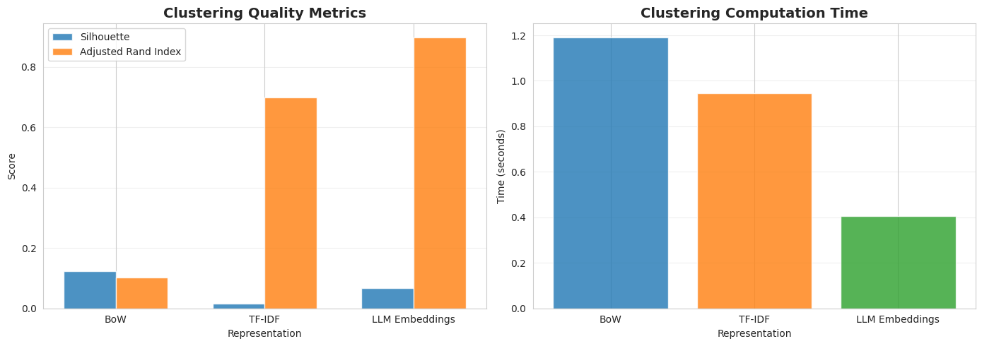
LLM embeddings gained this time, with an ARI rating of 0.899, exhibiting sturdy alignment between clusters discovered and actual subgroups that abide by true doc classes. That is largely as a result of clustering is an unsupervised studying activity and, not like classification, it is a territory the place semantic understanding like that offered by embeddings turns into much more essential for capturing patterns, even on less complicated datasets.
Abstract
Easier, well-behaved datasets like BBC information are an important instance of an issue the place superior and LLM-based representations like embeddings don’t all the time win. Conventional pure language processing approaches for textual content illustration could excel in issues with clear class boundaries, linear separability, and clear, formal textual content with out noisy patterns.
In sum, when addressing real-world machine studying tasks, think about all the time beginning with less complicated baselines and keyword-based representations like TF-IDF, earlier than straight leaping into state-of-the-art or most superior methods. The smaller your problem, the lighter the outfit you want to gown it with that excellent machine studying look!
On this article, you’ll learn the way Bag-of-Phrases, TF-IDF, and LLM-generated embeddings evaluate when used as textual content options for classification and clustering in scikit-learn.
Subjects we are going to cowl embody:
- Easy methods to generate Bag-of-Phrases, TF-IDF, and LLM embeddings for a similar dataset.
- How these representations evaluate on textual content classification efficiency and coaching pace.
- How they behave otherwise for unsupervised doc clustering.
Let’s get proper to it.
LLM Embeddings vs TF-IDF vs Bag-of-Phrases: Which Works Higher in Scikit-learn? (click on to enlarge)
Picture by Creator
Introduction
Machine studying fashions constructed with frameworks like scikit-learn can accommodate unstructured knowledge like textual content, so long as this uncooked textual content is transformed right into a numerical illustration that’s comprehensible by algorithms, fashions, and machines in a broader sense.
This text takes three well-known textual content illustration approaches — TF-IDF, Bag-of-Phrases, and LLM-generated embeddings — to supply an analytical and example-based comparability between them, within the context of downstream machine studying modeling with scikit-learn.
For a glimpse of textual content illustration approaches, together with an introduction to the three used on this article, we advocate you check out this text and this one.
The article will first navigate you thru a Python instance the place we are going to use the BBC information dataset — a labeled dataset containing a couple of thousand information articles categorized into 5 varieties — to acquire the three goal representations for every textual content, construct some textual content classifiers and evaluate them, and in addition construct and evaluate some clustering fashions. After that, we undertake a extra basic and analytical perspective to debate which method is best — and when to make use of one or one other.
Setup and Getting Textual content Representations
First, we import all of the modules and libraries we are going to want, arrange some configurations, and cargo the BBC information dataset:
|
1 2 3 4 5 6 7 8 9 10 11 12 13 14 15 16 17 18 19 20 21 22 23 24 25 26 27 28 29 30 31 32 33 34 35 |
import pandas as pd import numpy as np import matplotlib.pyplot as plt import seaborn as sns from time import time
# Scikit-learn imports from sklearn.feature_extraction.textual content import CountVectorizer, TfidfVectorizer from sklearn.model_selection import train_test_split, cross_val_score from sklearn.linear_model import LogisticRegression from sklearn.ensemble import RandomForestClassifier from sklearn.svm import SVC from sklearn.cluster import KMeans from sklearn.metrics import ( accuracy_score, f1_score, classification_report, silhouette_score, adjusted_rand_rating ) from sklearn.preprocessing import LabelEncoder
# Our key import for constructing LLM embeddings: a Sentence Transformer mannequin from sentence_transformers import SentenceTransformer
# Plotting configuration – for later analyzing and evaluating outcomes sns.set_style(“whitegrid”) plt.rcParams[‘figure.figsize’] = (14, 6)
# Loading BBC Information dataset print(“Loading BBC Information dataset…”) url = “https://storage.googleapis.com/dataset-uploader/bbc/bbc-text.csv” df = pd.read_csv(url)
print(f“Dataset loaded: {len(df)} paperwork”) print(f“Classes: {df[‘category’].distinctive()}”) print(f“nClass distribution:”) print(df[‘category’].value_counts()) |
On the time of writing, the dataset model we’re utilizing incorporates 2225 situations, that’s, paperwork containing information articles.
Since we are going to prepare some supervised machine studying fashions for classification in a while, earlier than acquiring the three representations for our textual content knowledge, we separate the enter texts from their labels and break up the entire dataset into coaching and take a look at subsets:
|
1 2 3 4 5 6 7 8 9 10 11 12 13 14 15 16 17 |
print(“n” + “=”*70) print(“DATA PREPARATION PRIOR TO GENERATING TEXT REPRESENTATIONS”) print(“=”*70)
texts = df[‘text’].tolist() labels = df[‘category’].tolist()
# Encoding labels for classification le = LabelEncoder() y = le.fit_transform(labels)
# Splitting knowledge (identical break up for all illustration strategies and ML fashions educated later) X_text_train, X_text_test, y_train, y_test = train_test_split( texts, y, test_size=0.2, random_state=42, stratify=y )
print(f“nTrain set: {len(X_text_train)} | Take a look at set: {len(X_text_test)}”) |
Illustration 1: Bag-of-Phrases (BoW)
|
1 2 3 4 5 6 7 8 9 10 11 12 13 14 15 16 17 18 19 |
print(“n[1] Bag-of-Phrases…”) begin = time()
# The CountVectorizer class is used to use BoW bow_vectorizer = CountVectorizer( max_features=5000, min_df=2, stop_words=‘english’ )
X_bow_train = bow_vectorizer.fit_transform(X_text_train) X_bow_test = bow_vectorizer.remodel(X_text_test)
bow_time = time() – begin
print(f” Performed in {bow_time:.2f}s”) print(f” Form: {X_bow_train.form} (paperwork × vocabulary)”) print(f” Sparsity: {(1 – X_bow_train.nnz / (X_bow_train.form[0] * X_bow_train.form[1])) * 100:.1f}%”) print(f” Reminiscence: {X_bow_train.knowledge.nbytes / 1024:.1f} KB”) |
Illustration 2: TF-IDF
|
1 2 3 4 5 6 7 8 9 10 11 12 13 14 15 16 17 18 19 |
print(“n[2] TF-IDF…”) begin = time()
# Utilizing TfidfVectorizer class to use TF-IDF primarily based on phrase frequencies tfidf_vectorizer = TfidfVectorizer( max_features=5000, min_df=2, stop_words=‘english’ )
X_tfidf_train = tfidf_vectorizer.fit_transform(X_text_train) X_tfidf_test = tfidf_vectorizer.remodel(X_text_test)
tfidf_time = time() – begin
print(f” Performed in {tfidf_time:.2f}s”) print(f” Form: {X_tfidf_train.form}”) print(f” Sparsity: {(1 – X_tfidf_train.nnz / (X_tfidf_train.form[0] * X_tfidf_train.form[1])) * 100:.1f}%”) print(f” Reminiscence: {X_tfidf_train.knowledge.nbytes / 1024:.1f} KB”) |
Illustration 3: LLM Embeddings
|
1 2 3 4 5 6 7 8 9 10 11 12 13 14 15 16 17 18 19 20 21 22 23 |
print(“n[3] LLM Embeddings…”) begin = time()
# Loading a pre-trained sentence transformer mannequin to generate 384-dimensional embeddings embedding_model = SentenceTransformer(‘all-MiniLM-L6-v2’)
X_emb_train = embedding_model.encode( X_text_train, show_progress_bar=True, batch_size=32 ) X_emb_test = embedding_model.encode( X_text_test, show_progress_bar=False, batch_size=32 )
emb_time = time() – begin
print(f” Performed in {emb_time:.2f}s”) print(f” Form: {X_emb_train.form} (paperwork × embedding_dim)”) print(f” Sparsity: 0.0% (dense illustration)”) print(f” Reminiscence: {X_emb_train.nbytes / 1024:.1f} KB”) |
Comparability 1: Textual content Classification
That was an intensive preparatory stage! Now we’re prepared for a primary comparability instance, centered on coaching a number of forms of machine studying classifiers and evaluating how every sort of classifier performs when educated on one textual content illustration or one other.
In a nutshell, the code offered under will:
- Take into account three classifier varieties: logistic regression, random forests, and assist vector machines (SVM).
- Practice and consider every of the three×3 = 9 classifiers educated, utilizing two analysis metrics: accuracy and F1 rating.
- Listing and visualize the outcomes obtained from every mannequin sort and textual content illustration method used.
|
1 2 3 4 5 6 7 8 9 10 11 12 13 14 15 16 17 18 19 20 21 22 23 24 25 26 27 28 29 30 31 32 33 34 35 36 37 38 39 40 41 42 43 44 45 46 47 48 49 50 51 52 53 |
print(“n” + “=”*70) print(“COMPARISON 1: SUPERVISED CLASSIFICATION”) print(“=”*70)
# Defining the three forms of classifiers to coach classifiers = { ‘Logistic Regression’: LogisticRegression(max_iter=1000, random_state=42), ‘Random Forest’: RandomForestClassifier(n_estimators=100, random_state=42), ‘SVM’: SVC(kernel=‘linear’, random_state=42) }
# Storing leads to a Python assortment (checklist) classification_results = []
# Evaluating every illustration with every classifier representations = { ‘BoW’: (X_bow_train, X_bow_test), ‘TF-IDF’: (X_tfidf_train, X_tfidf_test), ‘LLM Embeddings’: (X_emb_train, X_emb_test) }
for rep_name, (X_tr, X_te) in representations.gadgets(): print(f“nTesting {rep_name}:”) print(“-“ * 50)
for clf_name, clf in classifiers.gadgets(): # Practice begin = time() clf.match(X_tr, y_train) train_time = time() – begin
# Predict begin = time() y_pred = clf.predict(X_te) pred_time = time() – begin
# Consider acc = accuracy_score(y_test, y_pred) f1 = f1_score(y_test, y_pred, common=‘weighted’)
print(f” {clf_name:20s} | Acc: {acc:.3f} | F1: {f1:.3f} | Practice: {train_time:.2f}s”)
classification_results.append({ ‘Illustration’: rep_name, ‘Classifier’: clf_name, ‘Accuracy’: acc, ‘F1-Rating’: f1, ‘Practice Time’: train_time, ‘Predict Time’: pred_time })
# Changing outcomes to DataFrame for interpretability and simpler comparability results_df = pd.DataFrame(classification_results) |
Output:
|
1 2 3 4 5 6 7 8 9 10 11 12 13 14 15 16 17 18 19 20 21 |
====================================================================== COMPARISON 1: SUPERVISED CLASSIFICATION ======================================================================
Testing BoW: ————————————————————————— Logistic Regression | Acc: 0.982 | F1: 0.982 | Practice: 0.86s Random Forest | Acc: 0.973 | F1: 0.973 | Practice: 2.20s SVM | Acc: 0.984 | F1: 0.984 | Practice: 2.02s
Testing TF–IDF: ————————————————————————— Logistic Regression | Acc: 0.984 | F1: 0.984 | Practice: 0.52s Random Forest | Acc: 0.978 | F1: 0.977 | Practice: 1.79s SVM | Acc: 0.987 | F1: 0.987 | Practice: 2.99s
Testing LLM Embeddings: ————————————————————————— Logistic Regression | Acc: 0.982 | F1: 0.982 | Practice: 0.27s Random Forest | Acc: 0.960 | F1: 0.959 | Practice: 5.21s SVM | Acc: 0.980 | F1: 0.980 | Practice: 0.15s |
Enter code for visualizing outcomes:
|
1 2 3 4 5 6 7 8 9 10 11 12 13 14 15 16 17 18 19 20 21 22 23 24 25 26 27 28 29 30 31 32 33 |
# Creating visualization plots for direct comparability fig, axes = plt.subplots(1, 2, figsize=(16, 6))
# Plot 1: Accuracy comparability pivot_acc = results_df.pivot(index=‘Classifier’, columns=‘Illustration’, values=‘Accuracy’) pivot_acc.plot(sort=‘bar’, ax=axes[0], width=0.8) axes[0].set_title(‘Classification Accuracy by Illustration’, fontsize=14, fontweight=‘daring’) axes[0].set_ylabel(‘Accuracy’) axes[0].set_xlabel(‘Classifier’) axes[0].legend(title=‘Illustration’) axes[0].grid(axis=‘y’, alpha=0.3) axes[0].set_ylim([0.9, 1.0])
# Plot 2: Coaching time comparability pivot_time = results_df.pivot(index=‘Classifier’, columns=‘Illustration’, values=‘Practice Time’) pivot_time.plot(sort=‘bar’, ax=axes[1], width=0.8, colour=[‘#1f77b4’, ‘#ff7f0e’, ‘#2ca02c’]) axes[1].set_title(‘Coaching Time by Illustration’, fontsize=14, fontweight=‘daring’) axes[1].set_ylabel(‘Time (seconds)’) axes[1].set_xlabel(‘Classifier’) axes[1].legend(title=‘Illustration’) axes[1].grid(axis=‘y’, alpha=0.3)
plt.tight_layout() plt.present()
# Figuring out greatest performers print(“nBEST PERFORMERS:”) print(“-“ * 50) best_acc = results_df.loc[results_df[‘Accuracy’].idxmax()] print(f“Greatest Accuracy: {best_acc[‘Representation’]} + {best_acc[‘Classifier’]} = {best_acc[‘Accuracy’]:.3f}”)
quickest = results_df.loc[results_df[‘Train Time’].idxmin()] print(f“Quickest Coaching: {quickest[‘Representation’]} + {quickest[‘Classifier’]} = {quickest[‘Train Time’]:.2f}s”) |
Let’s take these outcomes with a pinch of salt, as they’re particular to the dataset and mannequin varieties educated, and not at all generalizable. TF-IDF mixed with an SVM classifier led to the perfect accuracy (0.987), whereas LLM embeddings with SVM yielded the quickest mannequin to coach (0.15s). In the meantime, the greatest total mixture when it comes to performance-speed steadiness is logistic regression with TF-IDF, with a virtually excellent accuracy of 0.984 and a really quick coaching time of 0.52s.
Why did LLM embeddings, supposedly probably the most superior of the three textual content illustration approaches, not present the perfect efficiency? There are a number of causes for this. First, the present 5 courses (information classes) within the BBC information dataset are strongly word-discriminative; in different phrases, they’re simply separable by class, so reasonably less complicated representations like TF-IDF are sufficient to seize these patterns very nicely. This additionally implies there’s no use for the deep semantic understanding that LLM embeddings obtain; in truth, this will typically be counterproductive and result in overfitting. As well as, due to the close to separability between information varieties, linear and less complicated fashions work nice, in comparison with advanced ones like random forests.
If we had a more difficult, real-world dataset than BBC information, with points like noise, paraphrasing, slang, and even cross-lingual knowledge, LLM embeddings would in all probability outperform the opposite two representations.
Concerning Bag-of-Phrases, on this situation it solely marginally outperforms when it comes to inference pace, so it’s primarily really useful for quite simple duties requiring most interpretability, or as a part of a baseline mannequin earlier than attempting different methods.
Comparability 2: Doc Clustering
We’ll think about a second situation: making use of k-means clustering with okay=5 and evaluating the cluster high quality throughout the three textual content illustration schemes. Discover within the code under that, since clustering is an unsupervised activity not requiring labels or train-test splitting, we are going to re-generate all three representations once more for the entire dataset.
|
1 2 3 4 5 6 7 8 9 10 11 12 13 14 15 16 17 18 19 20 21 22 23 24 25 26 27 28 29 30 31 32 33 34 35 36 37 38 39 40 41 42 43 44 45 46 47 48 49 |
print(“n” + “=”*70) print(“COMPARISON 2: DOCUMENT CLUSTERING”) print(“=”*70)
# Utilizing full dataset for clustering (no prepare/take a look at break up wanted) all_texts = texts all_labels = y
# Producing representations as soon as extra print(“nGenerating representations for full dataset…”)
X_bow_full = bow_vectorizer.fit_transform(all_texts) X_tfidf_full = tfidf_vectorizer.fit_transform(all_texts) X_emb_full = embedding_model.encode(all_texts, show_progress_bar=True, batch_size=32)
# Clustering with Okay-Means (okay=5, matching ground-truth classes) n_clusters = len(np.distinctive(all_labels)) clustering_results = []
representations_full = { ‘BoW’: X_bow_full, ‘TF-IDF’: X_tfidf_full, ‘LLM Embeddings’: X_emb_full }
for rep_name, X_full in representations_full.gadgets(): print(f“nClustering with {rep_name}:”)
begin = time() kmeans = KMeans(n_clusters=n_clusters, random_state=42, n_init=10) cluster_labels = kmeans.fit_predict(X_full) cluster_time = time() – begin
# Consider silhouette = silhouette_score(X_full, cluster_labels) ari = adjusted_rand_score(all_labels, cluster_labels)
print(f” Silhouette Rating: {silhouette:.3f}”) print(f” Adjusted Rand Index: {ari:.3f}”) print(f” Time: {cluster_time:.2f}s”)
clustering_results.append({ ‘Illustration’: rep_name, ‘Silhouette’: silhouette, ‘ARI’: ari, ‘Time’: cluster_time })
clustering_df = pd.DataFrame(clustering_results) |
Output:
|
Clustering with BoW: Silhouette Rating: 0.124 Adjusted Rand Index: 0.102 Time: 1.19s
Clustering with TF–IDF: Silhouette Rating: 0.016 Adjusted Rand Index: 0.698 Time: 0.94s
Clustering with LLM Embeddings: Silhouette Rating: 0.066 Adjusted Rand Index: 0.899 Time: 0.41s |
Code for visualizing outcomes:
|
1 2 3 4 5 6 7 8 9 10 11 12 13 14 15 16 17 18 19 20 21 22 23 24 25 26 27 28 29 30 31 |
# Creating comparability plots fig, axes = plt.subplots(1, 2, figsize=(14, 5))
# Plot 1: Clustering high quality metrics x = np.arange(len(clustering_df)) width = 0.35
axes[0].bar(x – width/2, clustering_df[‘Silhouette’], width, label=‘Silhouette’, alpha=0.8) axes[0].bar(x + width/2, clustering_df[‘ARI’], width, label=‘Adjusted Rand Index’, alpha=0.8) axes[0].set_xlabel(‘Illustration’) axes[0].set_ylabel(‘Rating’) axes[0].set_title(‘Clustering High quality Metrics’, fontsize=14, fontweight=‘daring’) axes[0].set_xticks(x) axes[0].set_xticklabels(clustering_df[‘Representation’]) axes[0].legend() axes[0].grid(axis=‘y’, alpha=0.3)
# Plot 2: Clustering time axes[1].bar(clustering_df[‘Representation’], clustering_df[‘Time’], colour=[‘#1f77b4’, ‘#ff7f0e’, ‘#2ca02c’], alpha=0.8) axes[1].set_xlabel(‘Illustration’) axes[1].set_ylabel(‘Time (seconds)’) axes[1].set_title(‘Clustering Computation Time’, fontsize=14, fontweight=‘daring’) axes[1].grid(axis=‘y’, alpha=0.3)
plt.tight_layout() plt.present()
print(“nBEST CLUSTERING PERFORMER:”) print(“-“ * 50) best_cluster = clustering_df.loc[clustering_df[‘ARI’].idxmax()] print(f“{best_cluster[‘Representation’]}: ARI = {best_cluster[‘ARI’]:.3f}, Silhouette = {best_cluster[‘Silhouette’]:.3f}”) |
LLM embeddings gained this time, with an ARI rating of 0.899, exhibiting sturdy alignment between clusters discovered and actual subgroups that abide by true doc classes. That is largely as a result of clustering is an unsupervised studying activity and, not like classification, it is a territory the place semantic understanding like that offered by embeddings turns into much more essential for capturing patterns, even on less complicated datasets.
Abstract
Easier, well-behaved datasets like BBC information are an important instance of an issue the place superior and LLM-based representations like embeddings don’t all the time win. Conventional pure language processing approaches for textual content illustration could excel in issues with clear class boundaries, linear separability, and clear, formal textual content with out noisy patterns.
In sum, when addressing real-world machine studying tasks, think about all the time beginning with less complicated baselines and keyword-based representations like TF-IDF, earlier than straight leaping into state-of-the-art or most superior methods. The smaller your problem, the lighter the outfit you want to gown it with that excellent machine studying look!


