


On this article, you’ll learn the way key-value (KV) caching eliminates redundant computation in autoregressive transformer inference to dramatically enhance era velocity.
Subjects we are going to cowl embody:
- Why autoregressive era has quadratic computational complexity
- How the eye mechanism produces question, key, and worth representations
- How KV caching works in follow, together with pseudocode and reminiscence trade-offs
Let’s get began.

KV Caching in LLMs: A Information for Builders
Picture by Editor
Introduction
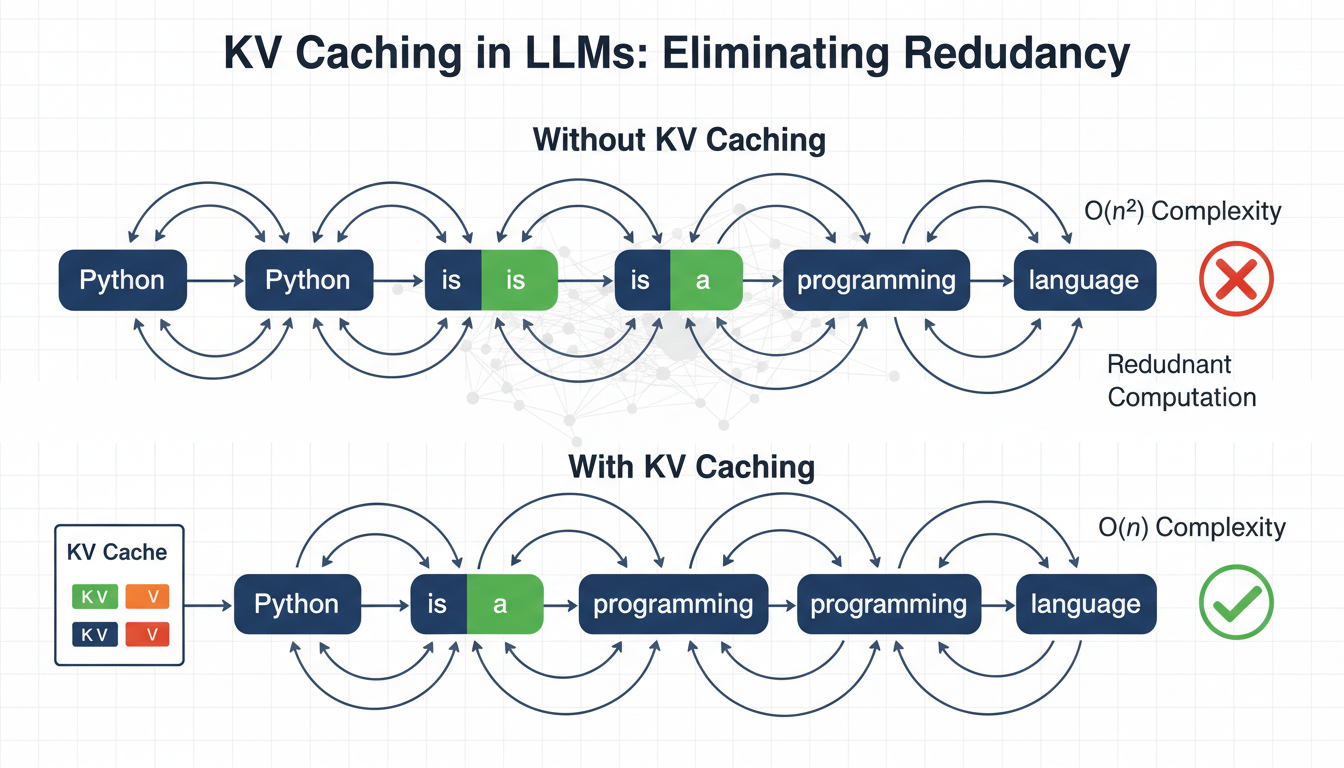
Language fashions generate textual content one token at a time, reprocessing all the sequence at every step. To generate token n, the mannequin recomputes consideration over all (n-1) earlier tokens. This creates ( O(n^2) ) complexity, the place computation grows quadratically with sequence size, which turns into a serious bottleneck for inference velocity.
Key-value (KV) caching eliminates this redundancy by leveraging the truth that the important thing and worth projections in consideration don’t change as soon as computed for a token. As an alternative of recomputing them at every step, we cache and reuse them. In follow, this could scale back redundant computation and supply 3–5× quicker inference, relying on mannequin dimension and {hardware}.
Conditions
This text assumes you’re aware of the next ideas:
- Neural networks and backpropagation
- The transformer structure
- The self-attention mechanism in transformers
- Matrix multiplication ideas resembling dot merchandise, transposes, and primary linear algebra
If any of those really feel unfamiliar, the sources under are good beginning factors earlier than studying on. The Illustrated Transformer by Jay Alammar is likely one of the clearest visible introductions to transformers and a focus accessible. Andrej Karpathy’s Let’s Construct GPT walks by way of constructing a transformer from scratch in code.
Each provides you with a strong basis to get probably the most out of this text. That stated, this text is written to be as self-contained as attainable, and plenty of ideas will change into clearer in context as you go.
The Computational Drawback in Autoregressive Era
Massive language fashions use autoregressive era — producing one token at a time — the place every token depends upon all earlier tokens.
Let’s use a easy instance. Begin with the enter phrase: “Python”. Suppose the mannequin generates:
|
Enter: “Python” Step 1: “is” Step 2: “a” Step 3: “programming” Step 4: “language” Step 5: “used” Step 6: “for” ... |
Right here is the computational downside: to generate “programming” (token 3), the mannequin processes “Python is a”. To generate “language” (token 4), it processes “Python is a programming”. Each new token requires reprocessing all earlier tokens.
Here’s a breakdown of tokens that get reprocessed repeatedly:
- “Python” will get processed 6 occasions (as soon as for every subsequent token)
- “is” will get processed 5 occasions
- “a” will get processed 4 occasions
- “programming” will get processed 3 occasions
The token “Python” by no means adjustments, but we recompute its inner representations time and again. On the whole, the method seems like this:
|
Generate token 1: Course of 1 place Generate token 2: Course of 2 positions Generate token 3: Course of 3 positions ... Generate token n: Course of n positions |
This provides us the next complexity for producing n tokens:
[
text{Cost} = 1 + 2 + 3 + cdots + n = frac{n(n+1)}{2} approx O(n^2)
]
Understanding the Consideration Mechanism and KV Caching
Consider consideration because the mannequin deciding which phrases to concentrate on. The self-attention mechanism on the core of transformers computes:
[
text{Attention}(Q, K, V) = text{softmax}left(frac{QK^T}{sqrt{d_k}}right)V
]
The mechanism creates three representations for every token:
- Question (Q): Every token makes use of its question to look the sequence for related context wanted to be interpreted appropriately.
- Key (Ok): Every token broadcasts its key so different queries can determine how related it’s to what they’re searching for.
- Worth (V): As soon as a question matches a key, the worth is what truly will get retrieved and used within the output.
Every token enters the eye layer as a ( d_{textual content{mannequin}} )-dimensional vector. The projection matrices ( W_Q ), ( W_K ), and ( W_V ) — realized throughout coaching by way of backpropagation — map it to ( d_k ) per head, the place ( d_k = d_{textual content{mannequin}} / textual content{num_heads} ).
Throughout coaching, the total sequence is processed without delay, so Q, Ok, and V all have form [seq_len, d_k], and ( QK^T ) produces a full [seq_len, seq_len] matrix with each token attending to each different token concurrently.
At inference, one thing extra attention-grabbing occurs. When producing token ( t ), solely Q adjustments. The Ok and V for all earlier tokens ( 1 ldots t-1 ) are equivalent to what they have been within the earlier step. Due to this fact, it’s attainable to cache these key (Ok) and worth (V) matrices and reuse them in subsequent steps. Therefore the identify KV caching.
Q has form [1, d_k] since solely the present token is handed in, whereas Ok and V have form [seq_len, d_k] and [seq_len, d_v], respectively, rising by one row every step as the brand new token’s Ok and V are appended.
With these shapes in thoughts, here’s what the components computes:
- ( QK^T ) computes a dot product between the present token’s question and each cached key, producing a
[1, seq_len]similarity rating throughout the total historical past. - ( 1/sqrt{d_k} ) scales scores down to forestall dot merchandise from rising too massive and saturating the softmax.
- ( textual content{softmax}(cdot) ) converts the scaled scores right into a likelihood distribution that sums to 1.
- Multiplying by V weights the worth vectors by these chances to supply the ultimate output.
Evaluating Token Era With and With out KV Caching
Let’s hint by way of our instance with concrete numbers. We are going to use ( d_{textual content{mannequin}} = 4 ). Actual fashions, nonetheless, sometimes use 768–4096 dimensions.
Enter: “Python” (1 token). Suppose the language mannequin generates: “is a programming language”.
With out KV Caching
At every step, Ok and V are recomputed for each token within the sequence, and the associated fee grows as every token is added.
| Step | Sequence | Ok & V Computed |
|---|---|---|
| 0 | Python | Python |
| 1 | Python is | Python, is |
| 2 | Python is a | Python, is, a |
| 3 | Python is a programming | Python, is, a, programming |
| 4 | Python is a programming language | Python, is, a, programming, language |
With KV Caching
With KV caching, solely the brand new token’s Ok and V are computed. All the things prior is retrieved instantly from the cache.
| Step | Sequence | Ok & V Computed & Cached | Ok & V Retrieved |
|---|---|---|---|
| 0 | Python | Python | — |
| 1 | Python is | is | Python |
| 2 | Python is a | a | Python, is |
| 3 | Python is a programming | programming | Python, is, a |
| 4 | Python is a programming language | language | Python, is, a, programming |
Implementing KV Caching: A Pseudocode Walkthrough
Initializing the Cache
The eye layer holds the cache as a part of its state. There are two slots for keys and values that begin empty and fill throughout era.
|
class MultiHeadAttentionWithCache: def __init__(self, d_model, num_heads): self.d_model = d_model self.num_heads = num_heads self.d_k = d_model // num_heads
# Discovered projection matrices self.W_Q = Linear(d_model, d_model) self.W_K = Linear(d_model, d_model) self.W_V = Linear(d_model, d_model) self.W_O = Linear(d_model, d_model)
# Cache storage (initially None) self.cache_K = None self.cache_V = None |
Solely Ok and V are cached. Q is at all times computed as a result of it represents the present question. Every layer within the mannequin maintains its personal impartial cache.
Utilizing Caching Logic within the Ahead Move
Earlier than any caching logic runs, the enter is projected into Q, Ok, and V and reshaped throughout consideration heads.
|
def ahead(self, x, use_cache=False): batch_size, seq_len, _ = x.form
Q = self.W_Q(x) K_new = self.W_K(x) V_new = self.W_V(x)
# [batch, seq_len, d_model] -> [batch, num_heads, seq_len, d_k] Q = reshape_to_heads(Q, self.num_heads) K_new = reshape_to_heads(K_new, self.num_heads) V_new = reshape_to_heads(V_new, self.num_heads) |
K_new and V_new symbolize solely the present enter. They haven’t been appended to the cache but. The reshape operation splits d_model evenly throughout heads so every head attends to a special subspace.
Updating the KV Cache
That is the important thing step. On the primary name, the cache is seeded, and on each subsequent name, new keys and values are appended to it.
|
if use_cache: if self.cache_K is None: self.cache_K = K_new self.cache_V = V_new else: self.cache_K = concat([self.cache_K, K_new], dim=2) self.cache_V = concat([self.cache_V, V_new], dim=2)
Ok = self.cache_Ok V = self.cache_V else: Ok = Ok_new V = V_new |
Concatenation occurs alongside dim=2, the sequence dimension, so the cache grows one token at a time. When caching is energetic, Ok and V at all times comprise the total historical past — which means each token the mannequin has seen on this session.
Computing Consideration
With Ok and V now containing the total historical past, consideration runs as ordinary. The one distinction is that seq_len_k is longer than seq_len_q throughout decoding.
|
scores = matmul(Q, transpose(Ok)) / sqrt(self.d_k) # scores: [batch, num_heads, seq_len_q, seq_len_k]
masks = create_causal_mask(Q.form[2], Ok.form[2]) scores = masked_fill(scores, masks == 0, –inf)
attn_weights = softmax(scores, dim=–1) output = matmul(attn_weights, V)
output = reshape_from_heads(output) output = self.W_O(output)
return output |
The causal masks ensures place ( i ) can solely attend to positions ( leq i ), preserving autoregressive order. The ultimate projection by way of W_O recombines all heads again right into a single ( d_{textual content{mannequin}} )-dimensional output.
Managing the Cache
Between era requests, the cache should be cleared as a result of stale keys and values from a earlier session can corrupt the subsequent.
|
def reset_cache(self): self.cache_K = None self.cache_V = None |
This could at all times be known as earlier than beginning a brand new era. Forgetting this can be a frequent supply of delicate, hard-to-debug points the place outputs seem contextually contaminated.
Producing Textual content
The era course of has two distinct phases: a parallel prefill over all the immediate, adopted by a sequential decode loop that provides one token at a time.
|
def generate_with_kv_cache(mannequin, input_ids, max_new_tokens): mannequin.reset_all_caches()
# Prefill: course of full immediate in parallel, populates cache logits = mannequin(input_ids, use_cache=True)
for _ in vary(max_new_tokens): next_token_logits = logits[:, –1, :] next_token = argmax(next_token_logits, keepdim=True) input_ids = concat([input_ids, next_token], dim=1)
# Solely the brand new token is handed — cache handles the remainder logits = mannequin(next_token, use_cache=True)
return input_ids |
Throughout prefill, the total immediate is processed in a single ahead cross, which fills the cache with Ok and V for each enter token. Throughout decoding, every step passes solely a single new token. The mannequin attends to all prior context by way of the cache, not by reprocessing it. That is why era scales effectively: compute per step stays fixed no matter how lengthy the sequence turns into.
To summarize why this works:
- Token 1: The mannequin sees
[input], and the cache shops Ok and V for the enter - Token 2: The mannequin sees
[token1], however consideration makes use of cached Ok and V from the enter as properly - Token 3: The mannequin sees
[token2], however consideration makes use of Ok and V fromenter,token1, andtoken2
As you may see, reminiscence grows linearly with sequence size, which may change into prohibitive for very lengthy contexts.
Wrapping Up
KV caching addresses a basic limitation in autoregressive textual content era, the place fashions repeatedly recompute consideration projections for beforehand processed tokens. By caching the important thing and worth matrices from the eye mechanism and reusing them throughout era steps, we remove redundant computation that may in any other case develop quadratically with sequence size.
This considerably quickens massive language mannequin inference. The trade-off is elevated reminiscence utilization, because the cache grows linearly with sequence size. In most real-world techniques, this reminiscence price is justified by the substantial enhancements in inference latency.
Understanding KV caching supplies a basis for extra superior inference optimizations. From right here, you may discover methods resembling quantized caches, sliding-window consideration, and speculative decoding to push efficiency even additional.
References & Additional Studying
On this article, you’ll learn the way key-value (KV) caching eliminates redundant computation in autoregressive transformer inference to dramatically enhance era velocity.
Subjects we are going to cowl embody:
- Why autoregressive era has quadratic computational complexity
- How the eye mechanism produces question, key, and worth representations
- How KV caching works in follow, together with pseudocode and reminiscence trade-offs
Let’s get began.
KV Caching in LLMs: A Information for Builders
Picture by Editor
Introduction
Language fashions generate textual content one token at a time, reprocessing all the sequence at every step. To generate token n, the mannequin recomputes consideration over all (n-1) earlier tokens. This creates ( O(n^2) ) complexity, the place computation grows quadratically with sequence size, which turns into a serious bottleneck for inference velocity.
Key-value (KV) caching eliminates this redundancy by leveraging the truth that the important thing and worth projections in consideration don’t change as soon as computed for a token. As an alternative of recomputing them at every step, we cache and reuse them. In follow, this could scale back redundant computation and supply 3–5× quicker inference, relying on mannequin dimension and {hardware}.
Conditions
This text assumes you’re aware of the next ideas:
- Neural networks and backpropagation
- The transformer structure
- The self-attention mechanism in transformers
- Matrix multiplication ideas resembling dot merchandise, transposes, and primary linear algebra
If any of those really feel unfamiliar, the sources under are good beginning factors earlier than studying on. The Illustrated Transformer by Jay Alammar is likely one of the clearest visible introductions to transformers and a focus accessible. Andrej Karpathy’s Let’s Construct GPT walks by way of constructing a transformer from scratch in code.
Each provides you with a strong basis to get probably the most out of this text. That stated, this text is written to be as self-contained as attainable, and plenty of ideas will change into clearer in context as you go.
The Computational Drawback in Autoregressive Era
Massive language fashions use autoregressive era — producing one token at a time — the place every token depends upon all earlier tokens.
Let’s use a easy instance. Begin with the enter phrase: “Python”. Suppose the mannequin generates:
|
Enter: “Python” Step 1: “is” Step 2: “a” Step 3: “programming” Step 4: “language” Step 5: “used” Step 6: “for” ... |
Right here is the computational downside: to generate “programming” (token 3), the mannequin processes “Python is a”. To generate “language” (token 4), it processes “Python is a programming”. Each new token requires reprocessing all earlier tokens.
Here’s a breakdown of tokens that get reprocessed repeatedly:
- “Python” will get processed 6 occasions (as soon as for every subsequent token)
- “is” will get processed 5 occasions
- “a” will get processed 4 occasions
- “programming” will get processed 3 occasions
The token “Python” by no means adjustments, but we recompute its inner representations time and again. On the whole, the method seems like this:
|
Generate token 1: Course of 1 place Generate token 2: Course of 2 positions Generate token 3: Course of 3 positions ... Generate token n: Course of n positions |
This provides us the next complexity for producing n tokens:
[
text{Cost} = 1 + 2 + 3 + cdots + n = frac{n(n+1)}{2} approx O(n^2)
]
Understanding the Consideration Mechanism and KV Caching
Consider consideration because the mannequin deciding which phrases to concentrate on. The self-attention mechanism on the core of transformers computes:
[
text{Attention}(Q, K, V) = text{softmax}left(frac{QK^T}{sqrt{d_k}}right)V
]
The mechanism creates three representations for every token:
- Question (Q): Every token makes use of its question to look the sequence for related context wanted to be interpreted appropriately.
- Key (Ok): Every token broadcasts its key so different queries can determine how related it’s to what they’re searching for.
- Worth (V): As soon as a question matches a key, the worth is what truly will get retrieved and used within the output.
Every token enters the eye layer as a ( d_{textual content{mannequin}} )-dimensional vector. The projection matrices ( W_Q ), ( W_K ), and ( W_V ) — realized throughout coaching by way of backpropagation — map it to ( d_k ) per head, the place ( d_k = d_{textual content{mannequin}} / textual content{num_heads} ).
Throughout coaching, the total sequence is processed without delay, so Q, Ok, and V all have form [seq_len, d_k], and ( QK^T ) produces a full [seq_len, seq_len] matrix with each token attending to each different token concurrently.
At inference, one thing extra attention-grabbing occurs. When producing token ( t ), solely Q adjustments. The Ok and V for all earlier tokens ( 1 ldots t-1 ) are equivalent to what they have been within the earlier step. Due to this fact, it’s attainable to cache these key (Ok) and worth (V) matrices and reuse them in subsequent steps. Therefore the identify KV caching.
Q has form [1, d_k] since solely the present token is handed in, whereas Ok and V have form [seq_len, d_k] and [seq_len, d_v], respectively, rising by one row every step as the brand new token’s Ok and V are appended.
With these shapes in thoughts, here’s what the components computes:
- ( QK^T ) computes a dot product between the present token’s question and each cached key, producing a
[1, seq_len]similarity rating throughout the total historical past. - ( 1/sqrt{d_k} ) scales scores down to forestall dot merchandise from rising too massive and saturating the softmax.
- ( textual content{softmax}(cdot) ) converts the scaled scores right into a likelihood distribution that sums to 1.
- Multiplying by V weights the worth vectors by these chances to supply the ultimate output.
Evaluating Token Era With and With out KV Caching
Let’s hint by way of our instance with concrete numbers. We are going to use ( d_{textual content{mannequin}} = 4 ). Actual fashions, nonetheless, sometimes use 768–4096 dimensions.
Enter: “Python” (1 token). Suppose the language mannequin generates: “is a programming language”.
With out KV Caching
At every step, Ok and V are recomputed for each token within the sequence, and the associated fee grows as every token is added.
| Step | Sequence | Ok & V Computed |
|---|---|---|
| 0 | Python | Python |
| 1 | Python is | Python, is |
| 2 | Python is a | Python, is, a |
| 3 | Python is a programming | Python, is, a, programming |
| 4 | Python is a programming language | Python, is, a, programming, language |
With KV Caching
With KV caching, solely the brand new token’s Ok and V are computed. All the things prior is retrieved instantly from the cache.
| Step | Sequence | Ok & V Computed & Cached | Ok & V Retrieved |
|---|---|---|---|
| 0 | Python | Python | — |
| 1 | Python is | is | Python |
| 2 | Python is a | a | Python, is |
| 3 | Python is a programming | programming | Python, is, a |
| 4 | Python is a programming language | language | Python, is, a, programming |
Implementing KV Caching: A Pseudocode Walkthrough
Initializing the Cache
The eye layer holds the cache as a part of its state. There are two slots for keys and values that begin empty and fill throughout era.
|
class MultiHeadAttentionWithCache: def __init__(self, d_model, num_heads): self.d_model = d_model self.num_heads = num_heads self.d_k = d_model // num_heads
# Discovered projection matrices self.W_Q = Linear(d_model, d_model) self.W_K = Linear(d_model, d_model) self.W_V = Linear(d_model, d_model) self.W_O = Linear(d_model, d_model)
# Cache storage (initially None) self.cache_K = None self.cache_V = None |
Solely Ok and V are cached. Q is at all times computed as a result of it represents the present question. Every layer within the mannequin maintains its personal impartial cache.
Utilizing Caching Logic within the Ahead Move
Earlier than any caching logic runs, the enter is projected into Q, Ok, and V and reshaped throughout consideration heads.
|
def ahead(self, x, use_cache=False): batch_size, seq_len, _ = x.form
Q = self.W_Q(x) K_new = self.W_K(x) V_new = self.W_V(x)
# [batch, seq_len, d_model] -> [batch, num_heads, seq_len, d_k] Q = reshape_to_heads(Q, self.num_heads) K_new = reshape_to_heads(K_new, self.num_heads) V_new = reshape_to_heads(V_new, self.num_heads) |
K_new and V_new symbolize solely the present enter. They haven’t been appended to the cache but. The reshape operation splits d_model evenly throughout heads so every head attends to a special subspace.
Updating the KV Cache
That is the important thing step. On the primary name, the cache is seeded, and on each subsequent name, new keys and values are appended to it.
|
if use_cache: if self.cache_K is None: self.cache_K = K_new self.cache_V = V_new else: self.cache_K = concat([self.cache_K, K_new], dim=2) self.cache_V = concat([self.cache_V, V_new], dim=2)
Ok = self.cache_Ok V = self.cache_V else: Ok = Ok_new V = V_new |
Concatenation occurs alongside dim=2, the sequence dimension, so the cache grows one token at a time. When caching is energetic, Ok and V at all times comprise the total historical past — which means each token the mannequin has seen on this session.
Computing Consideration
With Ok and V now containing the total historical past, consideration runs as ordinary. The one distinction is that seq_len_k is longer than seq_len_q throughout decoding.
|
scores = matmul(Q, transpose(Ok)) / sqrt(self.d_k) # scores: [batch, num_heads, seq_len_q, seq_len_k]
masks = create_causal_mask(Q.form[2], Ok.form[2]) scores = masked_fill(scores, masks == 0, –inf)
attn_weights = softmax(scores, dim=–1) output = matmul(attn_weights, V)
output = reshape_from_heads(output) output = self.W_O(output)
return output |
The causal masks ensures place ( i ) can solely attend to positions ( leq i ), preserving autoregressive order. The ultimate projection by way of W_O recombines all heads again right into a single ( d_{textual content{mannequin}} )-dimensional output.
Managing the Cache
Between era requests, the cache should be cleared as a result of stale keys and values from a earlier session can corrupt the subsequent.
|
def reset_cache(self): self.cache_K = None self.cache_V = None |
This could at all times be known as earlier than beginning a brand new era. Forgetting this can be a frequent supply of delicate, hard-to-debug points the place outputs seem contextually contaminated.
Producing Textual content
The era course of has two distinct phases: a parallel prefill over all the immediate, adopted by a sequential decode loop that provides one token at a time.
|
def generate_with_kv_cache(mannequin, input_ids, max_new_tokens): mannequin.reset_all_caches()
# Prefill: course of full immediate in parallel, populates cache logits = mannequin(input_ids, use_cache=True)
for _ in vary(max_new_tokens): next_token_logits = logits[:, –1, :] next_token = argmax(next_token_logits, keepdim=True) input_ids = concat([input_ids, next_token], dim=1)
# Solely the brand new token is handed — cache handles the remainder logits = mannequin(next_token, use_cache=True)
return input_ids |
Throughout prefill, the total immediate is processed in a single ahead cross, which fills the cache with Ok and V for each enter token. Throughout decoding, every step passes solely a single new token. The mannequin attends to all prior context by way of the cache, not by reprocessing it. That is why era scales effectively: compute per step stays fixed no matter how lengthy the sequence turns into.
To summarize why this works:
- Token 1: The mannequin sees
[input], and the cache shops Ok and V for the enter - Token 2: The mannequin sees
[token1], however consideration makes use of cached Ok and V from the enter as properly - Token 3: The mannequin sees
[token2], however consideration makes use of Ok and V fromenter,token1, andtoken2
As you may see, reminiscence grows linearly with sequence size, which may change into prohibitive for very lengthy contexts.
Wrapping Up
KV caching addresses a basic limitation in autoregressive textual content era, the place fashions repeatedly recompute consideration projections for beforehand processed tokens. By caching the important thing and worth matrices from the eye mechanism and reusing them throughout era steps, we remove redundant computation that may in any other case develop quadratically with sequence size.
This considerably quickens massive language mannequin inference. The trade-off is elevated reminiscence utilization, because the cache grows linearly with sequence size. In most real-world techniques, this reminiscence price is justified by the substantial enhancements in inference latency.
Understanding KV caching supplies a basis for extra superior inference optimizations. From right here, you may discover methods resembling quantized caches, sliding-window consideration, and speculative decoding to push efficiency even additional.


