Grad-CAM from Scratch with PyTorch Hooks

automotive stops all of a sudden. Worryingly, there isn’t a cease register sight. The engineers can solely make guesses as to why the automotive’s neural community grew to become confused. It could possibly be a tumbleweed rolling throughout the road, a automotive coming down the opposite lane or the purple billboard within the background. To search out the actual purpose, they flip to Grad-CAM [1].

Grad-CAM is an explainable AI (XAI) approach that helps reveal why a convolutional neural community (CNN) made a selected resolution. The tactic produces a heatmap that highlights the areas in a picture which can be crucial for a prediction. For our self-driving automotive instance, this might present if the pixels from the weed, automotive or billboard precipitated the automotive to cease.

Now, Grad-CAM is one among many XAI strategies for Pc Imaginative and prescient. Attributable to its velocity, flexibility and reliability, it has rapidly grow to be one of the fashionable. It has additionally impressed many associated strategies. So, in case you are enthusiastic about XAI, it’s price understanding precisely how this technique works. To try this, we might be implementing Grad-CAM from scratch utilizing Python.

Particularly, we might be counting on PyTorch Hooks. As you will notice, these enable us to dynamically extract gradients and activations from a community throughout ahead and backwards passes. These are sensible abilities that won’t solely assist you to implement Grad-CAM but in addition any gradient-based XAI technique. See the total undertaking on GitHub.

The idea behind Grad-CAM

Earlier than we get to the code, it’s price relating the speculation behind Grad-CAM. If you’d like a deep dive, then try the video under. If you wish to find out about different strategies, then see this free XAI for Pc Imaginative and prescient course.

To summarise, when creating Grad-CAM heatmaps, we begin with a skilled CNN. We then do a ahead move by way of this community with a single pattern picture. This can activate all convolutional layers within the community. We name these function maps ($A^ok$). They are going to be a group of 2D matrices that include totally different options detected within the pattern picture.

With Grad-CAM, we’re sometimes within the maps from the final convolutional layer of the community. Once we apply the strategy to VGG16, you will notice that its last layer has 512 function maps. We use these as they include options with essentially the most detailed semantic data whereas nonetheless retaining spatial data. In different phrases, they inform us what was used for a prediction and the place within the picture it was taken from.

The issue is that these maps additionally include options which can be vital for different courses. To mitigate this, we comply with the method proven in Determine 1. As soon as we now have the function maps ($A^ok$), we weight them by how vital they’re to the category of curiosity ($y_c$). We do that utilizing $a_k^c$ — the typical gradient of the rating for $y_c$ w.r.t. to the weather within the function map. We then do element-wise summation. For VGG16, you will notice we go from 512 maps of 14×14 pixels to a single 14×14 map.

The gradients for a person ingredient ($frac{partial y^c}{partial A_{ij}^ok}$) inform us how a lot the rating will change with a small change within the ingredient. Because of this massive common gradients point out that all the function map was vital and may contribute extra to the ultimate heatmap. So, after we weight and sum the maps, those that include options for different courses will probably contribute much less.

The ultimate steps are to use the ReLU activation perform to make sure all unfavorable parts can have a worth of zero. Then we upsample with interpolation so the heatmap has the identical dimensions because the pattern picture. The ultimate map is summarised by the method under. You would possibly recognise it from the Grad-CAM paper [1].

$$ L_{Grad-CAM}^c = ReLUleft( sum_{ok} a_k^c A^ok proper) $$

Grad-CAM from Scratch

Don’t fear if the speculation will not be fully clear. We are going to stroll by way of it step-by-step as we apply the strategy from scratch. You will discover the total undertaking on GitHub. To begin, we now have our imports under. These are all widespread imports for laptop imaginative and prescient issues.

import matplotlib.pyplot as plt
import numpy as np

import cv2
from PIL import Picture

import torch
import torch.nn.practical as F
from torchvision import fashions, transforms

import urllib.request

Load pretrained mannequin from PyTorch

We’ll be making use of Grad-CAM to VGG16 pretrained on ImageNet. To assist, we now have the 2 features under. The primary will format a picture within the right manner for enter into the mannequin. The normalisation values used are the imply and normal deviation of the pictures in ImageNet. The 224×224 dimension can be normal for ImageNet fashions.

def preprocess_image(img_path):

    """Load and preprocess pictures for PyTorch fashions."""

    img = Picture.open(img_path).convert("RGB")

    #Transforms utilized by imagenet fashions
    remodel = transforms.Compose([
        transforms.Resize((224, 224)),
        transforms.ToTensor(),
        transforms.Normalize(mean=[0.485, 0.456, 0.406], std=[0.229, 0.224, 0.225]),
    ])

    return remodel(img).unsqueeze(0)

ImageNet has many courses. The second perform will format the output of the mannequin so we show the courses with the very best predicted possibilities.

def display_output(output,n=5):

    """Show the highest n classes predicted by the mannequin."""
    
    # Obtain the classes
    url = "https://uncooked.githubusercontent.com/pytorch/hub/grasp/imagenet_classes.txt"
    urllib.request.urlretrieve(url, "imagenet_classes.txt")

    with open("imagenet_classes.txt", "r") as f:
        classes = [s.strip() for s in f.readlines()]

    # Present high classes per picture
    possibilities = torch.nn.practical.softmax(output[0], dim=0)
    top_prob, top_catid = torch.topk(possibilities, n)

    for i in vary(top_prob.dimension(0)):
        print(classes[top_catid[i]], top_prob[i].merchandise())

    return top_catid[0]

We now load the pretrained VGG16 mannequin (line 2), transfer it to a GPU (traces 5-8) and set it to analysis mode (line 11). You may see a snippet of the mannequin output in Determine 2. VGG16 is made from 16 weighted layers. Right here, you possibly can see the final 2 of 13 convolutional layers and the three absolutely linked layers.

# Load the pre-trained mannequin (e.g., VGG16)
mannequin = fashions.vgg16(pretrained=True)

# Set the mannequin to gpu
gadget = torch.gadget('mps' if torch.backends.mps.is_built() 
                      else 'cuda' if torch.cuda.is_available() 
                      else 'cpu')
mannequin.to(gadget)

# Set the mannequin to analysis mode
mannequin.eval()

The names you see in Determine 2 are vital. Later, we’ll use them to reference a selected layer within the community to entry its activations and gradients. Particularly, we’ll use mannequin.options[28]. That is the ultimate convolutional layer within the community. As you possibly can see within the snapshot, this layer comprises 512 function maps.

Ahead move with pattern picture

We might be explaining a prediction from this mannequin. To do that, we want a pattern picture that might be fed into the mannequin. We downloaded one from Wikipedia Commons (traces 2-3). We then load it (traces 5-6), crop it to have equal top and width (line 7) and show it (traces 9-10). In Determine 3, you possibly can see we’re utilizing a picture of a whale shark in an aquarium.

# Load a pattern picture from the net
img_url = "https://add.wikimedia.org/wikipedia/commons/thumb/a/a1/Male_whale_shark_at_Georgia_Aquarium.jpg/960px-Male_whale_shark_at_Georgia_Aquarium.jpg"
urllib.request.urlretrieve(img_url, "sample_image.jpg")[0]

img_path = "sample_image.jpg"
img = Picture.open(img_path).convert("RGB")
img = img.crop((320, 0, 960, 640))  # Crop to 640x640

plt.imshow(img)
plt.axis("off")

ImageNet has no devoted class for whale sharks, so will probably be attention-grabbing to see what the mannequin predicts. To do that, we begin by processing our picture (line 2) and transferring it to the GPU (line 3). We then do a ahead move to get a prediction (line 6) and show the highest 5 possibilities (line 7). You may see these in Determine 4.

# Preprocess the picture
img_tensor = preprocess_image(img_path)
img_tensor = img_tensor.to(gadget)

# Ahead move
predictions = mannequin(img_tensor)
display_output(predictions,n=5)

Given the obtainable courses, these appear affordable. They’re all marine life and the highest two are sharks. Now, let’s see how we are able to clarify this prediction. We need to perceive what areas of the picture contribute essentially the most to the very best predicted class — hammerhead.

PyTorch hooks naming conventions

Grad-CAM heatmaps are created utilizing each activations from a ahead move and gradients from a backwards move. To entry these, we’ll use PyTorch hooks. These are features that assist you to save the inputs and outputs of a layer. We gained’t do it right here, however they even assist you to alter these points. For instance, Guided Backpropagation will be utilized by making certain solely constructive gradients are propagated utilizing a backwards hook.

You may see some examples of those features under. A forwards_hook might be known as throughout a ahead move. Will probably be registered on a given module (i.e. layer). By default, the perform receives three arguments — the module, its enter and its output. Equally, a backwards_hook is triggered throughout a backwards move with the module and gradients of the enter and output.

# Instance of a forwards hook perform
def fowards_hook(module, enter, output):
    """Parameters:
            module (nn.Module): The module the place the hook is utilized.
            enter (tuple of Tensors): Enter to the module.
            output (Tensor): Output of the module."""
    ...

# Instance of a backwards hook perform 
def backwards_hook(module, grad_in, grad_out):
    """Parameters:
            module (nn.Module): The module the place the hook is utilized.
            grad_in (tuple of Tensors): Gradients w.r.t. the enter of the module.
            grad_out (tuple of Tensors): Gradients w.r.t. the output of the module."""
    ...

To keep away from confusion, let’s make clear the parameter names utilized by these features. Check out the overview of the usual backpropagation process for a convolutional layer in Determine 5. This layer consists of a set of kernels, $Okay$, and biases, $b$. The opposite components are the:

• enter – a set of function maps or a picture
• output – set of function maps
• grad_in is the gradient of the loss w.r.t. the layer’s enter.
• grad_out is the gradient of the loss w.r.t. the layer’s output.

Now we have labelled these utilizing the identical names of the arguments used to name the hook features that we apply later.

Consider, we gained’t use the gradients in the identical manner as backpropagation. Normally, we use the gradients of a batch of pictures to replace $Okay$ and $b$. Now, we’re solely enthusiastic about grad_out of a single pattern picture. This can give us the gradients of the weather within the layer’s function maps. In different phrases, the gradients we use to weight the function maps.

Activations with PyTorch ahead hook

Our VGG16 community has been created utilizing ReLU with inplace=True. These modify tensors in reminiscence, so the unique values are misplaced. That’s, tensors used as enter are overwritten by the ReLU perform. This will result in issues when making use of hooks, as we may have the unique enter. So we use the code under to exchange all ReLU features with inplace=False ones. This is not going to affect the output of the mannequin, however it can improve its reminiscence utilization.

# Exchange all in-place ReLU activations with out-of-place ones
def replace_relu(mannequin):

    for identify, baby in mannequin.named_children():
        if isinstance(baby, torch.nn.ReLU):
            setattr(mannequin, identify, torch.nn.ReLU(inplace=False))
            print(f"Changing ReLU activation in layer: {identify}")
        else:
            replace_relu(baby)  # Recursively apply to submodules

# Apply the modification to the VGG16 mannequin
replace_relu(mannequin)

Beneath we now have our first hook perform — save_activations. This can append the output from a module (line 6) to an inventory of activations (line 2). In our case, we’ll solely register the hook onto one module (i.e. the final convolutional layer), so this listing will solely include one ingredient. Discover how we format the output (line 6). We detach it from the computational graph so the community will not be affected. We additionally format them as a numpy array and squeeze the batch dimension.

# Listing to retailer activations
activations = []

# Perform to avoid wasting activations
def save_activations(module, enter, output):
    activations.append(output.detach().cpu().numpy().squeeze())

To make use of the hook perform, we register it on the final convolutional layer — mannequin.options[28]. That is achieved utilizing the register_forward_hook perform.

# Register the hook to the final convolutional layer
hook = mannequin.options[28].register_forward_hook(save_activations)

Now, after we do a ahead move (line 2), the save_activations hook perform might be known as for this layer. In different phrases, its output might be saved to the activations listing.

# Ahead move by way of the mannequin to get activations
prediction = mannequin(img_tensor)

Lastly, it’s good follow to take away the hook perform when it’s not wanted (line 2). This implies the ahead hook perform is not going to be triggered if we do one other ahead move.

# Take away the hook after use
hook.take away()  

The form of those activations is (512, 14, 14). In different phrases, we now have 512 function maps and every map is 14×14 pixels. You may see some examples of those in Determine 6. A few of these maps might include options vital for different courses or people who lower the chance of the anticipated class. So let’s see how we are able to discover gradients to assist establish crucial maps.

act_shape = np.form(activations[0])
print(f"Form of activations: {act_shape}") # (512, 14, 14)

Gradients with PyTorch backwards hooks

To get gradients, we comply with an identical course of to earlier than. The important thing distinction is that we now use the register_full_backward_hook to register the save_gradients perform (line 7). This can make sure that it’s known as throughout a backwards move. Importantly, we do the backwards move (line 16) from the output for the category with the very best rating (line 13). This successfully units the rating for this class to 1 and all different scores to 0. In different phrases, we get the gradients of the hammerhead class w.r.t. to the weather of the function maps.

gradients = []

def save_gradient(module, grad_in, grad_out):
    gradients.append(grad_out[0].cpu().numpy().squeeze())

# Register the backward hook on a convolutional layer
hook = mannequin.options[28].register_full_backward_hook(save_gradient)

# Ahead move
output = mannequin(img_tensor)

# Choose the category with highest rating
rating = output[0].max()

# Backward move from the rating
rating.backward()

# Take away the hook after use
hook.take away()

We can have a gradient for each ingredient of the function maps. So, once more, the form is (512, 14, 14). Determine 7 visualises a few of these. You may see some are likely to have increased values. Nonetheless, we’re not so involved with the person gradients. Once we create a Grad-CAM heatmap, we’ll use the typical gradient of every function map.

grad_shape = np.form(gradients[0])
print(f"Form of gradients: {grad_shape}") # (512, 14, 14)

Lastly, earlier than we transfer on, it’s good follow to reset the mannequin’s gradients (line 2). That is significantly vital when you plan to run the code for a number of pictures, as gradients will be gathered with every backwards move.

# Reset gradients
mannequin.zero_grad() 

Creating Grad-CAM heatmaps

First, we discover the imply gradients for every function map. There might be 512 of those common gradients. Plotting a histogram of them, you possibly can see most are typically round 0. In different phrases, these don’t have a lot affect on the anticipated rating. There are a number of that are likely to have a unfavorable affect and a constructive affect. It’s these function maps we need to give extra weight to.

# Step 1: mixture the gradients
gradients_aggregated = np.imply(gradients[0], axis=(1, 2))

We mix all of the activations by doing element-wise summation (traces 2-4). Once we do that, we weight every function map by its common gradient (line 3). In the long run, we can have one 14×14 array.

# Step 2: weight the activations by the aggregated gradients and sum them up
weighted_activations = np.sum(activations[0] * 
                              gradients_aggregated[:, np.newaxis, np.newaxis], 
                              axis=0)

These weighted activations will include each constructive and unfavorable pixels. We are able to contemplate the unfavorable pixels to be suppressing the anticipated rating. In different phrases, a rise within the worth of those areas tends to lower the rating. Since we’re solely within the constructive contributions—areas that help the category prediction—we apply a ReLU activation to the ultimate heatmap (line 2). You may see the distinction within the heatmaps in Determine 9.

# Step 3: ReLU summed activations
relu_weighted_activations = np.most(weighted_activations, 0)

You may see the heatmap in Determine 9 is kind of coarse. It will be extra helpful if it had the scale of the unique picture. That is why the final step for creating Grad-CAM heatmaps is to upsample to the dimension of the enter picture (traces 2-4). On this case, we now have a 224×224 picture.

#Step 4: Upsample the heatmap to the unique picture dimension
upsampled_heatmap = cv2.resize(relu_weighted_activations, 
                               (img_tensor.dimension(3), img_tensor.dimension(2)), 
                               interpolation=cv2.INTER_LINEAR)

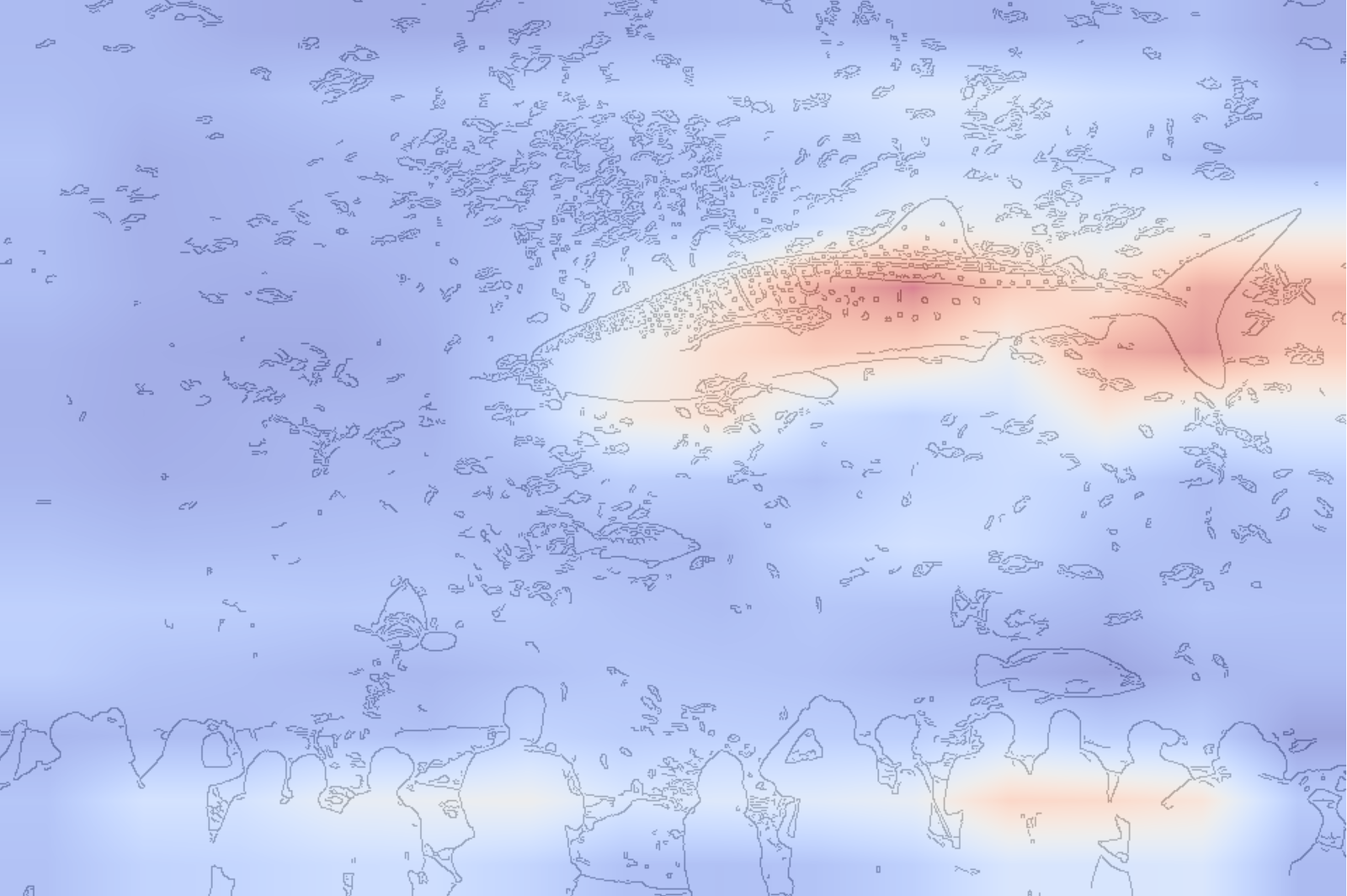
print(np.form(upsampled_heatmap))  # Needs to be (224, 224)

Determine 10 offers us our last visualisation. We show the pattern picture (traces 5-7) subsequent to the heatmap (traces 10-15). For the latter, we create a transparent visualisation with the assistance of Canny Edge detection (line 10). This provides us an edge map (i.e. define) of the pattern picture. We are able to then overlay the heatmap on high of this (line 14).

# Step 5: visualise the heatmap
fig, ax = plt.subplots(1, 2, figsize=(8, 8))

# Enter picture
resized_img = img.resize((224, 224))
ax[0].imshow(resized_img)
ax[0].axis("off")

# Edge map for the enter picture
edge_img = cv2.Canny(np.array(resized_img), 100, 200)
ax[1].imshow(255-edge_img, alpha=0.5, cmap='grey')

# Overlay the heatmap 
ax[1].imshow(upsampled_heatmap, alpha=0.5, cmap='coolwarm')
ax[1].axis("off")

Taking a look at our Grad-CAM heatmap, there’s some noise. Nonetheless, it seems the mannequin is counting on the tail fin and, to a lesser extent, the pectoral fin to make its predictions. It’s beginning to make sense why the mannequin categorised this shark as a hammerhead. Maybe each animals share these traits.

For some additional investigation, we apply the identical course of however now utilizing an precise picture of a hammerhead. On this case, the mannequin seems to be counting on the identical options. This can be a bit regarding. Would we not anticipate the mannequin to make use of one of many shark’s defining options— the hammerhead? In the end, this may occasionally lead VGG16 to confuse several types of sharks.

With this instance, we see how Grad-CAM can spotlight potential flaws in our mannequin. We can’t solely get their predictions but in addition perceive how they made them. We are able to perceive if the options used will result in unexpected predictions down the road. This will probably save us a whole lot of time, cash and within the case of extra consequential purposes, lives!

If you wish to be taught extra about XAI for CV try one among these articles. Or see this Free XAI for CV course.

References

[1] Ramprasaath R Selvaraju, Michael Cogswell, Abhishek Das, Ramakrishna Vedantam, Devi Parikh, and Dhruv Batra. Grad-cam: Visible explanations from deep networks through gradient-based localization. In Proceedings of the IEEE worldwide convention on laptop imaginative and prescient, pages 618–626, 2017.