


 Picture by Editor
# Introduction
Whereas knowledge preprocessing holds substantial relevance in knowledge science and machine studying workflows, these processes are sometimes not performed accurately, largely as a result of they’re perceived as overly complicated, time-consuming, or requiring in depth customized code. Consequently, practitioners could delay important duties like knowledge cleansing, depend on brittle ad-hoc options which are unsustainable in the long term, or over-engineer options to issues that may be easy at their core.
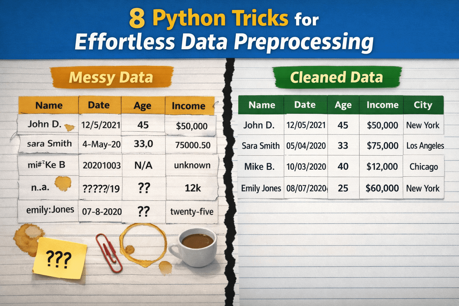
This text presents 8 Python methods to show uncooked, messy knowledge into clear, neatly preprocessed knowledge with minimal effort.
Earlier than wanting on the particular methods and accompanying code examples, the next preamble code units up the mandatory libraries and defines a toy dataset as an example every trick:
import pandas as pd
import numpy as np
# A tiny, deliberately messy dataset
df = pd.DataFrame({
    " Person Title ": [" Alice ", "bob", "Bob", "alice", None],
    "Age": ["25", "30", "?", "120", "28"],
    "Earnings$": ["50000", "60000", None, "1000000", "55000"],
    "Be part of Date": ["2023-01-01", "01/15/2023", "not a date", None, "2023-02-01"],
    "Metropolis": ["New York", "new york ", "NYC", "New York", "nyc"],
})
# 1. Normalizing Column Names Immediately
It is a very helpful, one-liner type trick: in a single line of code, it normalizes the names of all columns in a dataset. The specifics depend upon how precisely you need to normalize your attributes’ names, however the next instance exhibits learn how to substitute whitespaces with underscore symbols and lowercase every thing, thereby making certain a constant, standardized naming conference. That is vital to stop annoying bugs in downstream duties or to repair attainable typos. No must iterate column by column!
df.columns = df.columns.str.strip().str.decrease().str.substitute(" ", "_")
# 2. Stripping Whitespaces from Strings at Scale
Generally chances are you’ll solely need to be certain that particular junk invisible to the human eye, like whitespaces in the beginning or finish of string (categorical) values, is systematically eliminated throughout a complete dataset. This technique neatly does so for all columns containing strings, leaving different columns, like numeric ones, unchanged.
df = df.apply(lambda s: s.str.strip() if s.dtype == "object" else s)
# 3. Changing Numeric Columns Safely
If we’re not 100% certain that every one values in a numeric column abide by an similar format, it’s typically a good suggestion to explicitly convert these values to a numeric format, turning what may generally be messy strings wanting like numbers into precise numbers. In a single line, we are able to do what in any other case would require try-except blocks and a extra handbook cleansing process.
df["age"] = pd.to_numeric(df["age"], errors="coerce")
df["income$"] = pd.to_numeric(df["income$"], errors="coerce")
Observe right here that different classical approaches like df['columna'].astype(float) may generally crash if invalid uncooked values that can’t be trivially transformed into numeric have been discovered.
# 4. Parsing Dates with errors="coerce"
Comparable validation-oriented process, distinct knowledge sort. This trick converts date-time values which are legitimate, nullifying these that aren’t. Utilizing errors="coerce" is essential to inform Pandas that, if invalid, non-convertible values are discovered, they should be transformed into NaT (Not a Time), as an alternative of producing an error and crashing this system throughout execution.
df["join_date"] = pd.to_datetime(df["join_date"], errors="coerce")
# 5. Fixing Lacking Values with Good Defaults
For these unfamiliar with methods to deal with lacking values apart from dropping total rows containing them, this technique imputes these values — fills the gaps — utilizing statistically-driven defaults like median or mode. An environment friendly, one-liner-based technique that may be adjusted with totally different default aggregates. The [0] index accompanying the mode is used to acquire just one worth in case of ties between two or a number of “most frequent values”.
df["age"] = df["age"].fillna(df["age"].median())
df["city"] = df["city"].fillna(df["city"].mode()[0])
# 6. Standardizing Classes with Map
In categorical columns with various values, equivalent to cities, it’s also essential to standardize names and collapse attainable inconsistencies for acquiring cleaner group names and making downstream group aggregations like groupby() dependable and efficient. Aided by a dictionary, this instance applies a one-to-one mapping on string values associated to New York Metropolis, making certain all of them are uniformly denoted by “NYC”.
city_map = {"the big apple": "NYC", "nyc": "NYC"}
df["city"] = df["city"].str.decrease().map(city_map).fillna(df["city"])
# 7. Eradicating Duplicates Properly and Flexibly
The important thing for this extremely customizable duplicate removing technique is the usage of subset=["user_name"]. On this instance, it’s used to inform Pandas to deem a row as duplicated solely by wanting on the "user_name" column, and verifying whether or not the worth within the column is similar to the one in one other row. A good way to make sure each distinctive person is represented solely as soon as in a dataset, stopping double counting and doing all of it in a single instruction.
df = df.drop_duplicates(subset=["user_name"])
# 8. Clipping Quantiles for Outlier Removing
The final trick consists of capping excessive values or outliers robotically, as an alternative of solely eradicating them. Specifically helpful when outliers are assumed to be because of manually launched errors within the knowledge, as an example. Clipping units the acute values falling under (and above) two percentiles (1 and 99 within the instance), with such percentile values, maintaining authentic values mendacity between the 2 specified percentiles unchanged. In easy phrases, it’s like maintaining overly massive or small values inside the limits.
q_low, q_high = df["income$"].quantile([0.01, 0.99])
df["income$"] = df["income$"].clip(q_low, q_high)
# Wrapping Up
This text illustrated eight helpful methods, suggestions, and methods that may increase your knowledge preprocessing pipelines in Python, making them extra environment friendly, efficient, and sturdy: all on the similar time.
Iván Palomares Carrascosa is a pacesetter, author, speaker, and adviser in AI, machine studying, deep studying & LLMs. He trains and guides others in harnessing AI in the actual world.
Picture by Editor# Introduction
Whereas knowledge preprocessing holds substantial relevance in knowledge science and machine studying workflows, these processes are sometimes not performed accurately, largely as a result of they’re perceived as overly complicated, time-consuming, or requiring in depth customized code. Consequently, practitioners could delay important duties like knowledge cleansing, depend on brittle ad-hoc options which are unsustainable in the long term, or over-engineer options to issues that may be easy at their core.
This text presents 8 Python methods to show uncooked, messy knowledge into clear, neatly preprocessed knowledge with minimal effort.
Earlier than wanting on the particular methods and accompanying code examples, the next preamble code units up the mandatory libraries and defines a toy dataset as an example every trick:
import pandas as pd
import numpy as np
# A tiny, deliberately messy dataset
df = pd.DataFrame({
    " Person Title ": [" Alice ", "bob", "Bob", "alice", None],
    "Age": ["25", "30", "?", "120", "28"],
    "Earnings$": ["50000", "60000", None, "1000000", "55000"],
    "Be part of Date": ["2023-01-01", "01/15/2023", "not a date", None, "2023-02-01"],
    "Metropolis": ["New York", "new york ", "NYC", "New York", "nyc"],
})
# 1. Normalizing Column Names Immediately
It is a very helpful, one-liner type trick: in a single line of code, it normalizes the names of all columns in a dataset. The specifics depend upon how precisely you need to normalize your attributes’ names, however the next instance exhibits learn how to substitute whitespaces with underscore symbols and lowercase every thing, thereby making certain a constant, standardized naming conference. That is vital to stop annoying bugs in downstream duties or to repair attainable typos. No must iterate column by column!
df.columns = df.columns.str.strip().str.decrease().str.substitute(" ", "_")
# 2. Stripping Whitespaces from Strings at Scale
Generally chances are you’ll solely need to be certain that particular junk invisible to the human eye, like whitespaces in the beginning or finish of string (categorical) values, is systematically eliminated throughout a complete dataset. This technique neatly does so for all columns containing strings, leaving different columns, like numeric ones, unchanged.
df = df.apply(lambda s: s.str.strip() if s.dtype == "object" else s)
# 3. Changing Numeric Columns Safely
If we’re not 100% certain that every one values in a numeric column abide by an similar format, it’s typically a good suggestion to explicitly convert these values to a numeric format, turning what may generally be messy strings wanting like numbers into precise numbers. In a single line, we are able to do what in any other case would require try-except blocks and a extra handbook cleansing process.
df["age"] = pd.to_numeric(df["age"], errors="coerce")
df["income$"] = pd.to_numeric(df["income$"], errors="coerce")
Observe right here that different classical approaches like df['columna'].astype(float) may generally crash if invalid uncooked values that can’t be trivially transformed into numeric have been discovered.
# 4. Parsing Dates with errors="coerce"
Comparable validation-oriented process, distinct knowledge sort. This trick converts date-time values which are legitimate, nullifying these that aren’t. Utilizing errors="coerce" is essential to inform Pandas that, if invalid, non-convertible values are discovered, they should be transformed into NaT (Not a Time), as an alternative of producing an error and crashing this system throughout execution.
df["join_date"] = pd.to_datetime(df["join_date"], errors="coerce")
# 5. Fixing Lacking Values with Good Defaults
For these unfamiliar with methods to deal with lacking values apart from dropping total rows containing them, this technique imputes these values — fills the gaps — utilizing statistically-driven defaults like median or mode. An environment friendly, one-liner-based technique that may be adjusted with totally different default aggregates. The [0] index accompanying the mode is used to acquire just one worth in case of ties between two or a number of “most frequent values”.
df["age"] = df["age"].fillna(df["age"].median())
df["city"] = df["city"].fillna(df["city"].mode()[0])
# 6. Standardizing Classes with Map
In categorical columns with various values, equivalent to cities, it’s also essential to standardize names and collapse attainable inconsistencies for acquiring cleaner group names and making downstream group aggregations like groupby() dependable and efficient. Aided by a dictionary, this instance applies a one-to-one mapping on string values associated to New York Metropolis, making certain all of them are uniformly denoted by “NYC”.
city_map = {"the big apple": "NYC", "nyc": "NYC"}
df["city"] = df["city"].str.decrease().map(city_map).fillna(df["city"])
# 7. Eradicating Duplicates Properly and Flexibly
The important thing for this extremely customizable duplicate removing technique is the usage of subset=["user_name"]. On this instance, it’s used to inform Pandas to deem a row as duplicated solely by wanting on the "user_name" column, and verifying whether or not the worth within the column is similar to the one in one other row. A good way to make sure each distinctive person is represented solely as soon as in a dataset, stopping double counting and doing all of it in a single instruction.
df = df.drop_duplicates(subset=["user_name"])
# 8. Clipping Quantiles for Outlier Removing
The final trick consists of capping excessive values or outliers robotically, as an alternative of solely eradicating them. Specifically helpful when outliers are assumed to be because of manually launched errors within the knowledge, as an example. Clipping units the acute values falling under (and above) two percentiles (1 and 99 within the instance), with such percentile values, maintaining authentic values mendacity between the 2 specified percentiles unchanged. In easy phrases, it’s like maintaining overly massive or small values inside the limits.
q_low, q_high = df["income$"].quantile([0.01, 0.99])
df["income$"] = df["income$"].clip(q_low, q_high)
# Wrapping Up
This text illustrated eight helpful methods, suggestions, and methods that may increase your knowledge preprocessing pipelines in Python, making them extra environment friendly, efficient, and sturdy: all on the similar time.
Iván Palomares Carrascosa is a pacesetter, author, speaker, and adviser in AI, machine studying, deep studying & LLMs. He trains and guides others in harnessing AI in the actual world.


