


on Actual-World Issues is Laborious
Reinforcement studying appears easy in managed settings: well-defined states, dense rewards, stationary dynamics, limitless simulation. Most benchmark outcomes are produced below these assumptions. The true world violates almost all of them.
Observations are partial and noisy, rewards are delayed or ambiguous, environments drift over time, information assortment is gradual and costly, and errors carry actual value. Insurance policies should function below security constraints, restricted exploration, and non-stationary distributions. Off-policy information accumulates bias. Debugging is opaque. Small modeling errors compound into unstable habits.
Once more, reinforcement studying on actual world issues is actually arduous.
Exterior of managed simulators like Atari which reside in academia, there may be little or no sensible steerage on find out how to design, practice, or debug. Take away the assumptions that make benchmarks tractable and what stays is an issue area that appears close to unimaginable to really clear up.
However, then you might have these examples, and also you regain hope:
- OpenAI 5 defeated the reigning world champions in Dota 2 in full 5v5 matches. Educated utilizing deep reinforcement studying.
- DeepMind’s AlphaStar achieved Grandmaster rank in StarCraft II, surpassing 99.8% of human gamers and persistently defeating skilled rivals. Educated utilizing deep reinforcement studying.
- Boston Dynamic’s Atlas trains a 450M parameter Diffusion Transformer-based structure utilizing a mixture of actual world and simulated information. Educated utilizing deep reinforcement studying.
On this article, I’m going to introduce sensible, real-world approaches for coaching reinforcement studying brokers with parallelism, using many, if not the very same, strategies that energy right now’s superhuman AI techniques. This can be a deliberate number of educational strategies + hard-won expertise gained from constructing brokers which work on stochastic, nonstationary domains.
If you happen to intend on approaching a real-world drawback by merely making use of an untuned benchmark from an RL library on a single machine, you’ll probably fail.
One should perceive the next:
- Reframing the issue in order that it suits throughout the framework of RL concept
- The strategies for coverage optimization which really carry out outdoors of academia
- The nuances of “scale” with regard to reinforcement studying
Let’s start.
Stipulations
In case you have by no means approached reinforcement studying earlier than, making an attempt to construct a superhuman AI—or perhaps a midway first rate agent—is like making an attempt to show a cat to juggle flaming torches: it largely ignores you, often units one thing on fireplace, and someway you’re nonetheless anticipated to name it “progress.” Try to be nicely versed within the following topics:
- Markov Resolution Processes (MDPs) and Partially Observable Markov Resolution Processes (POMDPs): these present the mathematical basis for the way fashionable AI brokers work together with the world
- Coverage Optimization (in any other case often called Mirror Studying) Particulars as to how a neural community approximates an optimum coverage utilizing gradient ascent
- Comply with as much as 2) Actor Critic Strategies and Proximal Coverage Optimization (PPO), that are two broadly used strategies for coverage optimization
Every of those requires a while to completely perceive and digest. Sadly, RL is a troublesome drawback area, sufficient in order that merely scaling up is not going to clear up elementary misunderstandings or misapplications of the prerequisite steps as is typically the case in conventional deep studying.
An actual-world reinforcement studying drawback
To supply a coherent real-world instance, we use a simplified self-driving simulation because the optimization job. I say “simplified” as the precise particulars are much less necessary to the article’s goal. Nonetheless, for actual world RL, guarantee that you’ve got a full understanding of the setting, inputs, outputs and the way the reward is definitely generated. This understanding will show you how to body your actual world drawback into the area of MDPs.
Our simulator procedurally generates stochastic driving eventualities, together with pedestrians, different autos, and ranging terrain and street circumstances which have been modeled from recorded driving information. Every situation is segmented right into a variable-length episode.
Though many real-world issues aren’t true Markov Resolution Processes, they’re usually augmented in order that the efficient state is roughly Markov, permitting customary RL convergence ensures to carry roughly in follow.

States
The agent observes digicam and LiDAR inputs together with indicators corresponding to car velocity and orientation. Further options could embody the positions of close by autos and pedestrians. These observations are encoded as a number of tensors, optionally stacked over time to supply short-term historical past.
Actions
The motion area consists of steady car controls (steering, throttle, brake) and elective discrete controls (e.g., gear choice, flip indicators). Every motion is represented as a multidimensional vector specifying the management instructions utilized at every timestep.
Rewards
The reward encourages protected, environment friendly, and goal-directed driving. It combines a number of targets Oi, together with optimistic phrases for progress towards the vacation spot and penalties for collisions, site visitors violations, or unstable maneuvers. The per-timestep reward is a weighted sum:

We’ve constructed our simulation setting to suit throughout the 4 tuple interface popularized by Brockman et al., OpenAI Gymnasium, 2016
env = DrivingEnv()
agent = Agent()

for episode in vary(N):
   # obs is a multidimensional tensor representing the state
   obs = env.reset()
   finished = false

   whereas not finished:
       # act is the appliance of our present coverage π
       # π(obs) returns a multidimensional motion
       motion = agent.act(obs)
       # we ship the motion to the setting to obtain
       # the following step and reward till full
       next_obs, reward, finished, data = env.step(motion)
       obs = next_obs
The setting itself must be simply parallelized, such that one among many actors can concurrently apply their very own copy of the coverage with out the necessity for advanced interactions or synchronizations between brokers. This API, developed by OpenAI and used of their health club environments has turn out to be the defacto customary.
If you’re constructing your individual setting, it might be worthwhile to construct to this interface, because it simplifies many issues.
Agent
We use a deep actor–critic agent, following the method popularized in DeepMind’s A3C paper (Mnih et al., 2016). Pseudocode for our agent is beneath:
class Agent:
   def __init__(self, state_dim, action_dim):

       # --- Actor ---
       self.actor = Sequential(
           Linear(state_dim, 128),
           ReLU(),
           Linear(128, 128),
           ReLU(),
           Linear(128, action_dim)
       )

       # --- Critic ---
       self.critic = Sequential(
           Linear(state_dim, 128),
           ReLU(),
           Linear(128, 128),
           ReLU(),
           Linear(128, 1)
       )

   def _dist(self, state):
       logits = self.actor(state)
       return Categorical(logits=logits)

   def act(self, state):
       """
       Returns:
           motion
           log_prob (habits coverage)
           worth
       """
       dist = self._dist(state)

       motion = dist.pattern()
       log_prob = dist.log_prob(motion)
       worth = self.critic(state)

       return motion, log_prob, worth

   def log_prob(self, states, actions):
       dist = self._dist(states)
       return dist.log_prob(actions)

   def entropy(self, states):
       return self._dist(states).entropy()

   def worth(self, state):
       return self.critic(state)

   def replace(self, state_dict):
       self.actor.load_state_dict(state_dict['actor'])
       self.critic.load_state_dict(state_dict['critic'])
You could be a bit puzzled by the extra strategies. Extra clarification to observe.
Crucial be aware: Poorly chosen architectures can simply derail coaching. Ensure you perceive the motion area and confirm that your community’s enter, hidden, and output layers are appropriately sized and use appropriate activations.
Coverage Optimization
As a way to replace the agent, we observe the Proximal Coverage Optimization (PPO) framework (Schulman et al., 2017), which makes use of the clipped surrogate goal to replace the actor in a steady method whereas concurrently updating the critic. This enables the agent to enhance its coverage step by step based mostly on its collected expertise whereas holding updates inside a belief area, stopping massive, destabilizing coverage adjustments.
Word: PPO is likely one of the most generally used coverage optimization strategies, used to develop each OpenAI 5, Alphastar and lots of different actual world robotic management techniques
The agent first interacts with the setting, recording its actions, the rewards it receives, and its personal worth estimates. This sequence of expertise is often known as a rollout or, within the literature, a trajectory. The expertise could be collected to the tip of the episode, or extra generally, earlier than the episode ends for a set variety of steps. That is particularly helpful in infinite horizon issues with no predefined begin or end, because it permits for equal sized expertise batches from every actor.
Here’s a pattern rollout buffer. Nonetheless you select to design your buffer, It’s crucial that this rollout buffer be serializable in order that it may be despatched over the community.
class Rollout:
   def __init__(self):
       self.states = []
       self.actions = []
       # retailer logprob of motion!
       self.logprobs = []
       self.rewards = []
       self.values = []
       self.dones = []

   # Add a single timestep's expertise
   def add(self, state, motion, logprob, reward, worth, finished):
       self.states.append(state)
       self.actions.append(motion)
       self.logprobs.append(logprob)
       self.rewards.append(reward)
       self.values.append(worth)
       self.dones.append(finished)
   # Clear buffer after updates
   def reset(self):
       self.states = []
       self.actions = []
       self.logprobs = []
       self.rewards = []
       self.values = []
       self.dones = []
Throughout this rollout, the agent data states, actions, rewards, and subsequent states over a sequence of timesteps. As soon as the rollout is full, this expertise is used to compute the loss capabilities for each the actor and the critic.
Right here, we increase the agent setting interplay loop with our rollout buffer
env = DrivingEnv()
agent = Agent()
buffer = Rollout()

coach = Coach(agent)

rollout_steps = 256

for episode in vary(N):
   # obs is a multidimensional tensor representing the state
   obs = env.reset()
   finished = false
   steps = 0
   whereas not finished:
       steps += 1
       # act is the appliance of our present coverage π
       # π(obs) returns a multidimensional motion
       motion, logprob, worth = agent.act(obs)
       # we ship the motion to the setting to obtain
       # the following step and reward till full
       next_obs, reward, finished, data = env.step(motion)
       # add the expertise to the buffer
       buffer.add(state=obs, motion=motion, logprob=logprob, reward=reward,
                   worth=worth, finished=finished)
       if steps % rollout_steps == 0:
           # we'll add extra element right here
           state_dict = coach.practice(buffer)
           agent.replace(state_dict)
       obs = next_obs
I’m going to introduce the target perform as utilized in PPO, nonetheless, I do suggest studying the delightfully brief paper to get a full understanding of the nuances.
For the actor, we optimize a surrogate goal based mostly on the benefit perform, which measures how a lot better an motion carried out in comparison with the anticipated worth predicted by the critic.
The surrogate goal used to replace the actor community:

Word that the benefit, A, could be estimated in varied methods, corresponding to Generalized Benefit Estimation (GAE), or just utilizing the 1-step temporal-difference error, relying on the specified trade-off between bias and variance (Schulman et al., 2017).
The critic is up to date by minimizing the mean-squared error between its predicted worth V(s_t) and the noticed return R_t at every timestep. This trains the critic to precisely estimate the anticipated return of every state, which is then used to compute the benefit for the actor replace.

In PPO, the loss additionally contains an entropy part, which rewards insurance policies which have larger entropy. The rationale is {that a} coverage with larger entropy is extra random, encouraging the agent to discover a wider vary of actions slightly than prematurely converging to a deterministic habits. The entropy time period is often scaled by a coefficient, β, which controls the trade-off between exploration and exploitation.

The overall loss for PPO, then turns into:

Once more, in follow, merely utilizing the default parameters set forth within the baselines will go away you disgruntled and presumably psychotic after months of tedious hyperparameter tuning. As a way to prevent expensive journeys to the psychiatrist, please watch this very informative lecture by the creator of PPO, John Schulman. In it, he describes crucial particulars, corresponding to worth perform normalization, KL penalties, benefit normalization, and the way generally used strategies, like dropout and weight decay will poison your undertaking.
These particulars on this lecture, which aren’t laid out in any paper, are important to constructing a purposeful agent. Once more, as a cautious warning: for those who merely attempt to use the defaults with out understanding what is definitely taking place with coverage optimization, you’ll both fail or waste super time.
Our agent can now be up to date. Word that, since our optimizer is minimizing an goal, the indicators from the PPO goal as described within the paper have to be flipped.
Additionally be aware, that is the place our agent’s capabilities will come in useful.
def compute_advantages(rewards, values, gamma, lambda):
   # calc benefits as you would like

def compute_returns(rewards, gamma):
   # calc returns as you would like

def get_batches(buffer):
   # randomize and return tuples
   yield batch

class Coach:
   def __init__(self, agent, config):
       self.agent = agent                # ActorCriticAgent occasion
       self.lr = config.get("lr", 3e-4)
       self.num_epochs = config.get("num_epochs", 4)
       self.eps = config.get("clip_epsilon", 0.2)
       self.entropy_coeff = config.get("entropy_coeff", 0.01)
       self.value_loss_coeff = config.get("value_loss_coeff", 0.5)
       self.gamma = config.get("gamma", 0.99)
       self.lambda_gae = config.get("lambda", 0.95)

       # Single optimizer updating each actor and critic
       self.optimizer = Optimizer(params=checklist(agent.actor.parameters()) +
                                         checklist(agent.critic.parameters()),
                                  lr=self.lr)

   def practice(self, buffer):
       # --- 1. Compute benefits and returns ---
       benefits = compute_advantages(buffer.rewards, buffer.values, self.gamma, self.lambda_gae)
       returns = compute_returns(buffer.rewards, self.gamma)

       # --- 2. PPO updates ---
       for epoch in vary(self.num_epochs):
           for batch in get_batches(buffer):
               states, actions, adv, ret = batch

               # --- Likelihood ratio ---
               ratio = actor_prob(states, actions) / actor_prob_old(states, actions)

               # --- Actor loss (clipped surrogate) ---
               surrogate1 = ratio * adv
               surrogate2 = clip(ratio, 1 - self.eps, 1 + self.eps) * adv
               actor_loss = -mean(min(surrogate1, surrogate2))

               # --- Entropy bonus ---
               entropy = imply(policy_entropy(states))
               actor_loss -= self.entropy_coeff * entropy

               # --- Critic loss ---
               critic_loss = imply((critic_value(states) - ret) ** 2)

               # --- Whole PPO loss ---
               total_loss = actor_loss + self.value_loss_coeff * critic_loss

               # --- Apply gradients ---
               self.optimizer.zero_grad()
               total_loss.backward()
               self.optimizer.step()

        return self.agent.state_dict()
The three steps, defining our surroundings, defining our agent and its mannequin, in addition to defining our coverage optimization process are full and might now be used to construct an agent with a single machine.
Nothing described above will get you to “superhuman.”
Let’s wait for two months to your Macbook Professional with the overpriced M4 chip to begin exhibiting a 1% enchancment in efficiency (not kidding).
The Distributed Actor-Learner Structure
The actor–learner structure separates setting interplay from coverage optimization. Every actor operates independently, interacting with its personal setting utilizing a neighborhood copy of the coverage, which is mirrored throughout all actors. The learner doesn’t work together with the setting instantly; as a substitute, it serves as a centralized hub that updates the coverage and worth networks in response to the optimization goal and distributes the up to date fashions again to the actors.
This separation permits a number of actors to work together with the setting in parallel, bettering pattern effectivity and stabilizing coaching by decorrelating updates. This structure was popularized by DeepMind’s A3C paper (Mnih et al., 2016), which demonstrated that asynchronous actor–learner setups may practice large-scale reinforcement studying brokers effectively.

Actor
The actor is the part of the system that instantly interacts with the setting. Its tasks embody:
- Receiving a replica of the present coverage and worth networks from the learner.
- Sampling actions in response to the coverage for the present state of the setting.
- Accumulating expertise over a sequence of timesteps
- Sending the collected expertise to the learner asynchronously.
Learner
The learner is the centralized part chargeable for updating the mannequin parameters. Its tasks embody:
- Receiving expertise from a number of actors, both in full rollouts or in mini-batches.
- Computing loss capabilities
- Making use of gradient updates to the coverage and worth networks.
- Distributing the up to date mannequin again to actors, closing the loop.
This actor–learner separation just isn’t included in customary baselines corresponding to OpenAI Baselines or Secure Baselines. Whereas distributed actor–learner implementations do exist, for real-world issues the customization required could make the technical debt of adapting these frameworks outweigh the advantages of use.
Now issues are starting to get attention-grabbing.
With actors working asynchronously, whether or not on completely different elements of the identical episode or totally separate episodes our coverage optimization positive aspects a wealth of various experiences. On a single machine, this additionally means we are able to speed up expertise assortment dramatically, reducing coaching time proportionally to the variety of actors working in parallel.
Nonetheless, even the actor–learner structure is not going to get us to the dimensions we want as a result of a significant drawback: synchronization.
To ensure that the actors to start processing the following batch of expertise, all of them want to attend on the centralized learner to complete the coverage optimization step in order that the algorithm stays “on coverage.” This implies every actor is idle whereas the learner updates the mannequin utilizing the earlier batch of expertise, making a bottleneck that limits throughput and prevents totally parallelized information assortment.
Why not simply use previous batches from a coverage that was up to date a couple of step in the past?
Utilizing off-policy information to replace the mannequin has confirmed to be harmful. In follow, even small coverage lag introduces bias within the gradient estimate, and with perform approximation this bias can accumulate and trigger instability or outright divergence. This subject was noticed early in off-policy temporal-difference studying, the place bootstrapping plus perform approximation precipitated worth estimates to diverge as a substitute of converge, making naïve reuse of stale expertise unreliable at scale.
Fortunately, there’s a answer to this drawback.
IMPALA: Scalable Distributed Deep-RL with Significance Weighted Actor-Learner Architectures
Invented at DeepMind, IMPALA (and it’s predecessor, SEED-RL) launched an idea known as V-Hint, which permits us to replace on coverage algorithms with rollouts which have been generated off coverage.
Which means that the utilization of your complete system stays fixed, as a substitute of getting synchronization wait blocks (the actors want to attend for the newest mannequin replace as is the case in A3C). Nonetheless, this comes at a value: as a result of actors use barely stale parameters, trajectories are generated by older insurance policies, not the present learner coverage. Naively making use of on-policy strategies (e.g., customary coverage gradient or A2C) turns into biased and unstable.
To appropriate for this, we introduce V-Hint. V-Hint makes use of an importance-sampling–based mostly correction that adjusts returns to account for the mismatch between the habits coverage (actor) and goal coverage (learner).
In on-policy strategies, the beginning ratio (originally of every mini-epoch as is the case in PPO) is ~ 1. This implies the habits coverage is the same as the goal coverage.
In IMPALA, nonetheless, actors constantly generate expertise utilizing barely stale parameters, so trajectories are sampled from a habits coverage μ which will differ nontrivially from the learner’s present coverage π. Merely put, the beginning ratio != 1. This significance weight, permits us to approximate how stale the coverage which generated the expertise is.
We solely want yet another calculation to appropriate for this off-policy drift, which is to calculate the ratio of the habits coverage μ, in comparison with the present coverage, π at first of the coverage replace. We are able to then recalculate the coverage loss and worth targets utilizing a clipped variations of those significance weights — rho for the coverage and c for the worth targets.

We then recalculate our td-error (delta):

Then, use this worth to calculate our significance weighted values.

Now that we now have pattern corrected values, we have to recalculate our benefits.

Intuitively, V-trace compares how possible every sampled motion is below the present coverage versus the previous coverage that generated it.
If the motion remains to be probably below the brand new coverage, the ratio is close to one and the pattern is trusted.
If the motion is now unlikely, the ratio is small and its affect is lowered.
As a result of the ratio is clipped at one, samples can by no means be upweighted — solely downweighted — so stale or mismatched trajectories step by step lose impression whereas near-on-policy rollouts dominate the educational sign.
This crucial set of strategies permits us to extract all the horsepower from our coaching infrastructure and fully removes the bottleneck from synchronization. We not want to attend for all of the actors to complete their rollouts, losing expensive GPU + CPU time.
Given this technique, We have to make some modifications to our actor learner structure to take benefit.
Massively Distributed Actor-Learner Structure
As described above, we are able to nonetheless use our Distributed Actor-Learner structure, nonetheless, we have to add a number of parts and use some strategies from NVIDIA to permit for trajectories and weights to be obtained with none want for synchronization primitives or a central supervisor.

Key-Worth (KV) Database
Right here, we add a easy KV database like Redis to retailer trajectories. The addition requires us to serialize every trajectory after an actor completes gathering expertise, then every actor can merely add it to a Redis checklist. Redis is thread protected, so we don’t want to fret about synchronization for every actor.
When the learner is prepared for a brand new replace, it could possibly merely pop the newest trajectories off of this checklist, merge them, and carry out the coverage optimization process.
# modifying our actor steps
r = redis.Redis(...)Py

...

if steps % rollout_steps == 0:
 # as a substitute of coaching, simply serialize and ship to a buffer
 buffer_data = pickle.dumps(buffer)
 r.rpush("trajectories", buffer_data)


The learner can merely seize trajectories in a batch as wanted from this checklist,
which updates the weights.


# on the learner
trajectories = []

whereas len(trajectories) <= trajectory_batch_size:
 trajectory = pickle.masses(r.lpop("trajectories"))
 trajectories.append(trajectory)

# we are able to merge these right into a single buffer for the needs of coaching
buffer = merge_trajectories(trajectories)

# proceed coaching
A number of Learners (elective)
When you might have tons of of staff, a single GPU on the learner can turn out to be a bottleneck. This could trigger the trajectories to be very off-policy, which degrades studying efficiency. Nonetheless, so long as every learner runs the identical code (similar backward passes), they will every course of fully completely different trajectories independently.
Beneath the hood, in case you are utilizing PyTorch, NVIDIA’s NCCL library handles the all-reduce operations required to synchronize gradients. This ensures that mannequin weights stay constant throughout all learners. You’ll be able to launch every learner course of utilizing torchrun, which manages the distributed execution and coordination of the gradient updates robotically.
import torch.distributed as dist

r = redis.Redis(..)

def setup(rank, world_size):
   # Initialize the default course of group
   dist.init_process_group(
       backend="nccl",
       init_method=os.environ["MASTER_ADDR"],  # will set in launch command
       rank=rank,
       world_size=world_size
   )
   torch.cuda.set_device(rank % torch.cuda.device_count())

# apply coaching as above
...

total_loss = actor_loss + self.value_loss_coeff * critic_loss

# making use of our coaching step above
self.optimizer.zero_grad()
total_loss.backward()
# we have to use a dist operatiom
for p in agent.parameters():
  dist.all_reduce(p.grad.information)
  p.grad.information /= world_size

optimizer.step()
if rank == 0:
  # replace params from the grasp
  r.rpush("params", agent.get_state_dict())
I’m dramatically oversimplifying the appliance of NCCL. Learn the PyTorch documentation concerning distributed coaching
Assuming we use 2 nodes, every with 2 learners —
On node 1:
MASTER_ADDR={use your ip}
MASTER_PORT={decide an unused port}
WORLD_SIZE=4
RANK=0
torchrun --nnodes=2 --nproc_per_node=2
--rdzv_backend=c10d --rdzv_endpoint={your ADDR}:{your port} learner.py
and on node 2:
MASTER_ADDR={use your ip}
MASTER_PORT={decide an unused port}
WORLD_SIZE=4
RANK=2
torchrun --nnodes=2 --nproc_per_node=2
--rdzv_backend=c10d --rdzv_endpoint={your ADDR}:{your port} learner.py
Wrapping up
In abstract, scaling reinforcement studying from single-node experiments to distributed, multi-machine setups isn’t just a efficiency optimization—it’s a necessity for tackling advanced, real-world duties.
We coated:
- The way to refactor drawback areas into an MDP
- Agent structure
- Coverage optimization strategies that really work
- Scaling up distributed information assortment and coverage optimization
By combining a number of actors to gather various trajectories, fastidiously synchronizing learners with strategies like V-trace and all-reduce, and effectively coordinating computation throughout GPUs and nodes, we are able to practice brokers that method or surpass human-level efficiency in environments far tougher than basic benchmarks.
Mastering these methods bridges the hole between analysis on “toy” issues and constructing RL techniques able to working in wealthy, dynamic domains, from superior video games to robotics and autonomous techniques.
References
- Vinyals, O., Babuschkin, I., Czarnecki, W. M., Mathieu, M., Dudzik, A., Chung, J., … & Silver, D. (2019). Grandmaster stage in StarCraft II utilizing multi‑agent reinforcement studying. Nature.
- Berner, C., Brockman, G., Chan, B., Cheung, V., Dębiak, P., Dennison, C., … & Salimans, T. (2019). Dota 2 with massive scale deep reinforcement studying. arXiv:1912.06680
- Mnih, V., Kavukcuoglu, Ok., Silver, D., Rusu, A.A., Veness, J., Bellemare, M.G., … & Hassabis, D. (2015). Human-level management via deep reinforcement studying. Nature, 518(7540), 529–533.
- Schulman, J., Levine, S., Moritz, P., Jordan, M., & Abbeel, P. (2015). Belief Area Coverage Optimization. ICML 2015.
- Schulman, J., Wolski, F., Dhariwal, P., Radford, A., & Klimov, O. (2017). Proximal Coverage Optimization Algorithms. arXiv:1707.06347.
- Espeholt, L., Soyer, H., Munos, R., Simonyan, Ok., Mnih, V., Ward, T., … & Kavukcuoglu, Ok. (2018). IMPALA: Scalable Distributed Deep-RL with Significance Weighted Actor-Learner Architectures. ICML 2018.
- Espeholt, L., Stooke, A., Ibarz, J., Leibo, J.Z., Zambaldi, V., Tune, F., … & Silver, D. (2020). SEED RL: Scalable and Environment friendly Deep-RL with Accelerated Centralized Studying. arXiv:1910.06591.


