


is the method of choosing an optimum subset of options from a given set of options; an optimum function subset is the one which maximizes the efficiency of the mannequin on the given job.
Function choice could be a handbook or slightly specific course of when carried out with filter or wrapper strategies. In these strategies, options are added or eliminated iteratively based mostly on the worth of a hard and fast measure, which quantifies the relevance of the function within the making the prediction. The measures may very well be data achieve, variance or the chi-squared statistic, and the algorithm would decide to simply accept/reject the function contemplating a hard and fast threshold on the measure. Word, these strategies are usually not part of the mannequin coaching stage and are carried out previous to it.
Embedded strategies carry out function choice implicitly, with out utilizing any pre-defined choice standards and deriving it from the coaching information itself. This intrinsic function choice course of is part of the mannequin coaching stage. The mannequin learns to pick out options and make related predictions on the identical time. In later sections, we are going to describe the function of regularization in performing this intrinsic function choice.
Regularization and Mannequin Complexity
Regularization is the method of penalizing the complexity of the mannequin to keep away from overfitting and obtain generalization over the job.
Right here, the complexity of the mannequin is analogous to its energy to adapt to the patterns within the coaching information. Assuming a easy polynomial mannequin in ‘x’ with diploma ‘d’, as we improve the diploma ‘d’ of the polynomial, the mannequin achieves higher flexibility to seize patterns within the noticed information.
Overfitting and Underfitting
If we try to suit a polynomial mannequin with d = 2 on a set of coaching samples which have been derived from a cubic polynomial with some noise, the mannequin will be unable to seize the distribution of the samples to a ample extent. The mannequin merely lacks the flexibility or complexity to mannequin the info generated from a level 3 (or larger order) polynomials. Such a mannequin is claimed to under-fit on the coaching information.
Engaged on the identical instance, assume we now have a mannequin with d = 6. Now with elevated complexity, it needs to be simple for the mannequin to estimate the unique cubic polynomial that was used to generate the info (like setting the coefficients of all phrases with exponent > 3 to 0). If the coaching course of is just not terminated on the proper time, the mannequin will proceed to make the most of its extra flexibility to scale back the error inside additional and begin capturing within the noisy samples too. This can cut back the coaching error considerably, however the mannequin now overfits the coaching information. The noise will change in real-world settings (or within the take a look at part) and any information based mostly on predicting them will disrupt, resulting in excessive take a look at error.
The right way to decide the optimum mannequin complexity?
In sensible settings, we’ve little-to-no understanding of the data-generation course of or the true distribution of the info. Discovering the optimum mannequin with the appropriate complexity, such that no under-fitting or overfitting happens is a problem.
One method may very well be to start out with a sufficiently highly effective mannequin after which cut back its complexity by the use of function choice. Lesser the options, lesser is the complexity of the mannequin.
As mentioned within the earlier part, function choice might be specific (filter, wrapper strategies) or implicit. Redundant options which have insignificant relevance within the figuring out the worth of the response variable needs to be eradicated to keep away from the mannequin studying uncorrelated patterns in them. Regularization, additionally performs an analogous job. So, how are regularization and have choice linked to realize a typical purpose of optimum mannequin complexity?
L1 Regularization As A Function Selector
Persevering with with our polynomial mannequin, we symbolize it as a perform f, with inputs x, parameters θ and diploma d,

For a polynomial mannequin, every energy of the enter x_i might be thought-about as a function, forming a vector of the shape,

We additionally outline an goal perform, which on minimizing leads us to the optimum parameters θ* and features a regularization time period penalizing the complexity of the mannequin.

To find out the minima of this perform, we have to analyze all of its essential factors i.e. factors the place the derivation is zero or undefined.
The partial by-product w.r.t. one the parameters, θj, might be written as,

the place the perform sgn is outlined as,

Word: The by-product of absolutely the perform is totally different from the sgn perform outlined above. The unique by-product is undefined at x = 0. We increase the definition to take away the inflection level at x = 0 and to make the perform differentiable throughout its total area. Furthermore, such augmented capabilities are additionally utilized by ML frameworks when the underlying computation entails absolutely the perform. Verify this thread on the PyTorch discussion board.
By computing the partial by-product of the target perform w.r.t. a single parameter θj, and setting it to zero, we are able to construct an equation that relates the optimum worth of θj with the predictions, targets, and options.


Allow us to study the equation above. If we assume that the inputs and targets have been centered in regards to the imply (i.e. the info had been standardized within the preprocessing step), the time period on the LHS successfully represents the covariance between the jth function and the distinction between the anticipated and goal values.
Statistical covariance between two variables quantifies how a lot one variable influences the worth of the second variable (and vice-versa)
The signal perform on the RHS forces the covariance on the LHS to imagine solely three values (because the signal perform solely returns -1, 0 and 1). If the jth function is redundant and doesn’t affect the predictions, the covariance will likely be practically zero, bringing the corresponding parameter θj* to zero. This ends in the function being eradicated from the mannequin.
Think about the signal perform as a canyon carved by a river. You’ll be able to stroll within the canyon (i.e. the river mattress) however to get out of it, you could have these big limitations or steep slopes. L1 regularization induces an analogous ‘thresholding’ impact for the gradient of the loss perform. The gradient should be highly effective sufficient to interrupt the limitations or develop into zero, which ultimately brings the parameter to zero.
For a extra grounded instance, think about a dataset that comprises samples derived from a straight line (parameterized by two coefficients) with some added noise. The optimum mannequin shouldn’t have any greater than two parameters, else it should adapt to the noise current within the information (with the added freedom/energy to the polynomial). Altering the parameters of the upper powers within the polynomial mannequin doesn’t have an effect on the distinction between the targets and the mannequin’s predictions, thus lowering their covariance with the function.
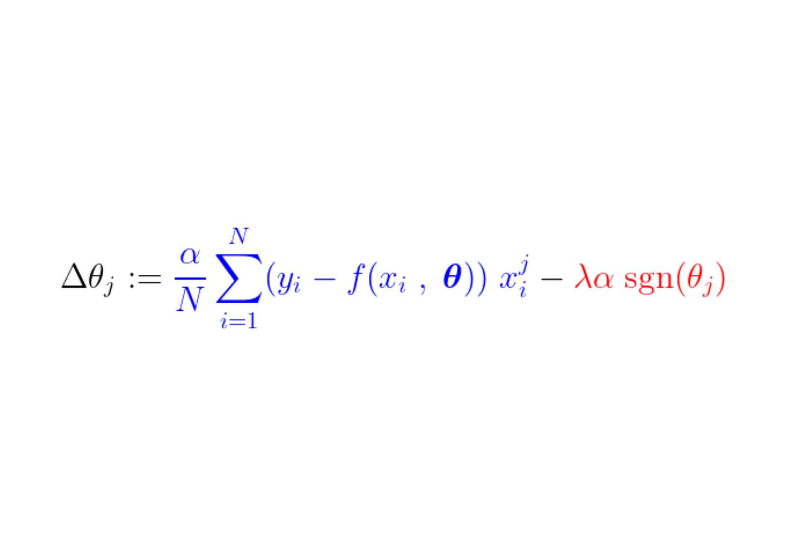
In the course of the coaching course of, a relentless step will get added/subtracted from the gradient of the loss perform. If the gradient of the loss perform (MSE) is smaller than the fixed step, the parameter will ultimately attain to a price of 0. Observe the equation under, depicting how parameters are up to date with gradient descent,


If the blue half above is smaller than λα, which itself is a really small quantity, Δθj is the practically a relentless step λα. The signal of this step (purple half) relies on sgn(θj), whose output relies on θj. If θj is constructive i.e. higher than ε, sgn(θj) equals 1, therefore making Δθj approx. equal to –λα pushing it in direction of zero.
To suppress the fixed step (purple half) that makes the parameter zero, the gradient of the loss perform (blue half) needs to be bigger than the step measurement. For a bigger loss perform gradient, the worth of the function should have an effect on the output of the mannequin considerably.
That is how a function is eradicated, or extra exactly, its corresponding parameter, whose worth doesn’t correlate with the output of the mannequin, is zero-ed by L1 regularization in the course of the coaching.
Additional Studying And Conclusion
- To get extra insights on the subject, I’ve posted a query on r/MachineLearning subreddit and the ensuing thread comprises totally different explanations that you could be need to learn.
- Madiyar Aitbayev additionally has an attention-grabbing weblog overlaying the identical query, however with a geometrical clarification.
- Brian Keng’s weblog explains regularization from a probabilistic perspective.
- This thread on CrossValidated explains why L1 norm encourages sparse fashions. An in depth weblog by Mukul Ranjan explains why L1 norm encourages the parameters to develop into zero and never the L2 norm.
“L1 regularization performs function choice” is a straightforward assertion that the majority ML learners agree with, with out diving deep into the way it works internally. This weblog is an try and convey my understanding and mental-model to the readers with a view to reply the query in an intuitive method. For solutions and doubts, yow will discover my electronic mail at my web site. Continue to learn and have a pleasant day forward!


