Constructing Sturdy Credit score Scoring Fashions with Python

you to your suggestions and curiosity in my earlier article. Since a number of readers requested learn how to replicate the evaluation, I made a decision to share the complete code on GitHub for each this text and the earlier one. This can will let you simply reproduce the outcomes, higher perceive the methodology, and discover the venture in additional element.

On this submit, we present that analyzing the relationships between variables in credit score scoring serves two essential functions:

• Evaluating the power of explanatory variables to discriminate default (see part 1.1)
• Decreasing dimensionality by finding out the relationships between explanatory variables (see part 1.2)
• In Part 1.3, we apply these strategies to the dataset launched in our earlier submit.
• In conclusion, we summarize the important thing takeaways and spotlight the details that may be helpful for interviews, whether or not for an internship or a full-time place.

As we develop and enhance our modeling abilities, we regularly look again and smile at our early makes an attempt, the primary fashions we constructed, and the errors we made alongside the way in which.

I keep in mind constructing a scoring mannequin utilizing Kaggle assets with out actually understanding learn how to analyze relationships between variables. Whether or not it concerned two steady variables, a steady and a categorical variable, or two categorical variables, I lacked each the graphical instinct and the statistical instruments wanted to review them correctly.

It wasn’t till my third 12 months, throughout a credit score scoring venture, that I totally grasped their significance. That have is why I strongly encourage anybody constructing their first scoring mannequin to take the evaluation of relationships between variables critically.

Why Finding out Relationships Between Variables Issues

The primary goal is to determine the variables that finest clarify the phenomenon underneath examine, for instance, predicting default.

Nonetheless, correlation is just not causation. Any perception have to be supported by:

• tutorial analysis
• area experience
• knowledge visualization
• and professional judgment

The second goal is dimensionality discount. By defining applicable thresholds, we are able to preselect variables that present significant associations with the goal or with different predictors. This helps scale back redundancy and enhance mannequin efficiency.

It additionally supplies early steering on which variables are prone to be retained within the ultimate mannequin and helps detect potential modeling points. For example, if a variable with no significant relationship to the goal leads to the ultimate mannequin, this will likely point out a weak point within the modeling course of. In such instances, you will need to revisit earlier steps and determine doable shortcomings.

On this article, we deal with three forms of relationships:

• Two steady variables
• One steady and one qualitative variable
• Two qualitative variables

All analyses are carried out on the coaching dataset. In a earlier article, we addressed outliers and lacking values, a vital prerequisite earlier than any statistical evaluation. Due to this fact, we are going to work with a cleaned dataset to investigate relationships between variables.

Outliers and lacking values can considerably distort each statistical measures and visible interpretations of relationships. Because of this it’s crucial to make sure that preprocessing steps, equivalent to dealing with lacking values and outliers, are carried out rigorously and appropriately.

The objective of this text is to not present an exhaustive checklist of statistical exams for measuring associations between variables. As a substitute, it goals to provide the important foundations wanted to grasp the significance of this step in constructing a dependable scoring mannequin.

The strategies introduced listed here are among the many mostly utilized in follow. Nonetheless, relying on the context, analysts might depend on extra or extra superior methods.

By the tip of this text, you need to have the ability to confidently reply the next three questions, which are sometimes requested in internships or job interviews:

• How do you measure the connection between two steady variables?
• How do you measure the connection between two qualitative variables?
• How do you measure the connection between a qualitative variable and a steady variable?

Graphical Evaluation

I initially wished to skip this step and go straight to statistical testing. Nonetheless, since this text is meant for learners in modeling, that is arguably crucial half.

At any time when you’ve gotten the chance to visualise your knowledge, you need to take it. Visualization can reveal an ideal deal concerning the underlying construction of the information, typically greater than a single statistical metric.

This step is especially crucial throughout the exploratory section, in addition to throughout decision-making and discussions with area consultants. The insights derived from visualizations ought to at all times be validated by:

• material consultants
• the context of the examine
• and related tutorial or scientific literature

By combining these views, we are able to eradicate variables that aren’t related to the issue or which will result in deceptive conclusions. On the similar time, we are able to determine essentially the most informative variables that actually assist clarify the phenomenon underneath examine.

When this step is rigorously executed and supported by tutorial analysis and professional validation, we are able to have larger confidence within the statistical exams that observe, which finally summarize the data into indicators equivalent to p-values or correlation coefficients.

In credit score scoring, the target is to pick out, from a set of candidate variables, those who finest clarify the goal, usually default.

Because of this we examine relationships between variables.

We are going to see later that some fashions are delicate to multicollinearity, which happens when a number of variables carry comparable data. Decreasing redundancy is due to this fact important.

In our case, the goal variable is binary (default vs. non-default), and we purpose to discriminate it utilizing explanatory variables that could be both steady or categorical.

Graphically, we are able to assess the discriminative energy of those variables, that’s, their capacity to foretell the default consequence. Within the following part, we current graphical strategies and take a look at statistics that may be automated to investigate the connection between steady or categorical explanatory variables and the goal variable, utilizing programming languages equivalent to Python.

1.1 Analysis of Predictive Energy

On this part, we current the graphical and statistical instruments used to evaluate the power of each steady and categorical explanatory variables to seize the connection with the goal variable, specifically default (def).

1.1.1 Steady Variable vs. Binary Goal

If the variable we’re evaluating is steady, the objective is to match its distribution throughout the 2 goal courses:

• non-default ($def = 0$)
• default ($def = 1$)

We are able to use:

• boxplots to match medians and dispersion
• density plots (KDE) to match distributions
• cumulative distribution capabilities (ECDF)

The important thing concept is straightforward:

Does the distribution of the variable differ between defaulters and non-defaulters?

If the reply is sure, the variable might have discriminative energy.

Assume we need to assess how nicely person_income discriminates between defaulting and non-defaulting debtors. Graphically, we are able to evaluate abstract statistics such because the imply or median, in addition to the distribution by density plots or cumulative distribution capabilities (CDFs) for defaulted and non-defaulted counterparties. The ensuing visualization is proven under.

def plot_continuous_vs_categorical(
    df,
    continuous_var,
    categorical_var,
    category_labels=None,
    figsize=(12, 10),
    pattern=None
):
    """
     Examine a steady variable throughout classes
    utilizing boxplot, KDE, and ECDF (2x2 format).
    """

    sns.set_style("white")

    knowledge = df[[continuous_var, categorical_var]].dropna().copy()

    # Optionally available sampling
    if pattern:
        knowledge = knowledge.pattern(pattern, random_state=42)

    classes = sorted(knowledge[categorical_var].distinctive())

    # Labels mapping (optionally available)
    if category_labels:
        labels = [category_labels.get(cat, str(cat)) for cat in categories]
    else:
        labels = [str(cat) for cat in categories]

    fig, axes = plt.subplots(2, 2, figsize=figsize)

    # --- 1. Boxplot ---
    sns.boxplot(
        knowledge=knowledge,
        x=categorical_var,
        y=continuous_var,
        ax=axes[0, 0]
    )
    axes[0, 0].set_title("Boxplot (median & unfold)", loc="left")

    # --- 2. Boxplot comparaison médianes ---
    sns.boxplot(
        knowledge=knowledge,
        x=categorical_var,
        y=continuous_var,
        ax=axes[0, 1],
        showmeans=True,
        meanprops={
            "marker": "o",
            "markerfacecolor": "white",
            "markeredgecolor": "black",
            "markersize": 6
        }
    )

    axes[0, 1].set_title("Median comparability (Boxplot)", loc="left")
    medians = knowledge.groupby(categorical_var)[continuous_var].median()

    for i, cat in enumerate(classes):
        axes[0, 1].textual content(
            i,
            medians[cat],
            f"{medians[cat]:.2f}",
            ha='heart',
            va='backside',
            fontsize=10,
            fontweight='daring'
        )
    # --- 3. KDE solely ---
    for cat, label in zip(classes, labels):
        subset = knowledge[data[categorical_var] == cat][continuous_var]
        sns.kdeplot(
            subset,
            ax=axes[1, 0],
            label=label
        )
    axes[1, 0].set_title("Density comparability (KDE)", loc="left")
    axes[1, 0].legend()

    # --- 4. ECDF ---
    for cat, label in zip(classes, labels):
        subset = np.type(knowledge[data[categorical_var] == cat][continuous_var])
        y = np.arange(1, len(subset) + 1) / len(subset)
        axes[1, 1].plot(subset, y, label=label)
    axes[1, 1].set_title("Cumulative distribution (ECDF)", loc="left")
    axes[1, 1].legend()

    # Clear type (Storytelling with Knowledge)
    for ax in axes.flat:
        sns.despine(ax=ax)
        ax.grid(axis="y", alpha=0.2)

    plt.tight_layout()
    plt.present()

plot_continuous_vs_categorical(
    df=train_imputed,
    continuous_var="person_income",
    categorical_var="def",
    category_labels={0: "No Default", 1: "Default"},
    figsize=(14, 12),
    pattern=5000
)

Defaulted debtors are likely to have decrease incomes than non-defaulted debtors. The distributions present a transparent shift, with defaults concentrated at decrease earnings ranges. General, earnings has good discriminatory energy for predicting default.

1.1.2 Statistical Check: Kruskal–Wallis for a Steady Variable vs. a Binary Goal

To formally assess this relationship, we use the Kruskal–Wallis take a look at, a non-parametric methodology.
It evaluates whether or not a number of unbiased samples come from the identical distribution.

Extra exactly, it exams whether or not ok samples (ok ≥ 2) originate from the identical inhabitants, or from populations with equivalent traits by way of a place parameter. This parameter is conceptually near the median, however the Kruskal–Wallis take a look at incorporates extra data than the median alone.

The precept of the take a look at is as follows. Let ($M_i$) denote the place parameter of pattern i. The hypotheses are:

• $( H_0 ): ( M_1 = dots = M_k )$
• $( H_1 )$: There exists a minimum of one pair (i, j) such that $( M_i neq M_j )$

When ( ok = 2 ), the Kruskal–Wallis take a look at reduces to the Mann–Whitney U take a look at.

The take a look at statistic roughly follows a Chi-square distribution with Ok-1 levels of freedom (for sufficiently giant samples).

• If the p-value < 5%, we reject $H_0$
• This means that a minimum of one group differs considerably

Due to this fact, for a given quantitative explanatory variable, if the p-value is lower than 5%, the null speculation is rejected, and we might conclude that the thought of explanatory variable could also be predictive within the mannequin.

1.1.3 Qualitative Variable vs. Binary Goal

If the explanatory variable is qualitative, the suitable instrument is the contingency desk, which summarizes the joint distribution of the 2 variables.

It reveals how the classes of the explanatory variable are distributed throughout the 2 courses of the goal. For instance the connection between person_home_ownership and the default variable, the contingency desk is given by :

def contingency_analysis(
    df,
    var1,
    var2,
    normalize=None,   # None, "index", "columns", "all"
    plot=True,
    figsize=(8, 6)
):
    """
    perform to compute and visualize contingency desk
    + Chi-square take a look at + Cramér's V.
    """

    # --- Contingency desk ---
    desk = pd.crosstab(df[var1], df[var2], margins=False)

    # --- Normalized model (optionally available) ---
    if normalize:
        table_norm = pd.crosstab(df[var1], df[var2], normalize=normalize, margins=False).spherical(3) * 100
    else:
        table_norm = None

    # --- Plot (heatmap) ---
    if plot:
        sns.set_style("white")
        plt.determine(figsize=figsize)

        data_to_plot = table_norm if table_norm is just not None else desk

        sns.heatmap(
            data_to_plot,
            annot=True,
            fmt=".2f" if normalize else "d",
            cbar=True
        )

        plt.title(f"{var1} vs {var2} (Contingency Desk)", loc="left", weight="daring")
        plt.xlabel(var2)
        plt.ylabel(var1)

        sns.despine()
        plt.tight_layout()
        plt.present()

  

From this desk, we are able to:

• Examine conditional distributions throughout classes.

• Debtors who hire or fall into “different” classes default extra typically, whereas householders have the bottom default fee.
  Mortgage holders are in between, suggesting average danger.

For visualization, grouped bar charts are sometimes used. They supply an intuitive strategy to evaluate conditional proportions throughout classes.

def plot_grouped_bar(df, cat_var, subcat_var,
                          normalize="index", title=""):
    ct = pd.crosstab(df[subcat_var], df[cat_var], normalize=normalize) * 100
    modalities = ct.index.tolist()
    classes = ct.columns.tolist()
    n_mod = len(modalities)
    n_cat = len(classes)
    x = np.arange(n_mod)
    width = 0.35

    colours = ['#0F6E56', '#993C1D']  # teal = non-défaut, coral = défaut

    fig, ax = plt.subplots(figsize=(7.24, 4.07), dpi=100)

    for i, (cat, colour) in enumerate(zip(classes, colours)):
        offset = (i - n_cat / 2 + 0.5) * width
        ax.bar(x + offset, ct[cat], width=width, colour=colour, label=str(cat))

        # Annotations au-dessus de chaque barre
        for j, val in enumerate(ct[cat]):
            ax.textual content(x[j] + offset, val + 0.5, f"{val:.1f}%",
                    ha='heart', va='backside', fontsize=9, colour='#444')

    # Type Cole
    ax.spines['top'].set_visible(False)
    ax.spines['right'].set_visible(False)
    ax.spines['left'].set_visible(False)
    ax.yaxis.grid(True, colour='#e0e0e0', linewidth=0.8, zorder=0)
    ax.set_axisbelow(True)
    ax.set_xticks(x)
    ax.set_xticklabels(modalities, fontsize=11)
    ax.set_ylabel("Taux (%)" if normalize else "Effectifs", fontsize=11, colour='#555')
    ax.tick_params(left=False, colours='#555')


    handles = [mpatches.Patch(color=c, label=str(l))
               for c, l in zip(colors, categories)]
    ax.legend(handles=handles, title=cat_var, frameon=False,
              fontsize=10, loc='higher proper')

    ax.set_title(title, fontsize=13, fontweight='regular', pad=14)
    plt.tight_layout()
    plt.savefig("default_by_ownership.png", dpi=150, bbox_inches='tight')
    plt.present()

plot_grouped_bar(
    df=train_imputed,
    cat_var="def",
    subcat_var="person_home_ownership",
    normalize="index",
    title="Default Price by Dwelling Possession"
)

1.1.4 Statistical Check: Evaluation of the Hyperlink Between Default and Qualitative Explanatory Variables

The statistical take a look at used is the chi-square take a look at, which is a take a look at of independence.
It goals to match two variables in a contingency desk to find out whether or not they’re associated. Extra usually, it assesses whether or not the distributions of categorical variables differ from one another.

A small chi-square statistic signifies that the noticed knowledge are near the anticipated knowledge underneath independence. In different phrases, there isn’t a proof of a relationship between the variables.

Conversely, a big chi-square statistic signifies a larger discrepancy between noticed and anticipated frequencies, suggesting a possible relationship between the variables. If the p-value of the chi-square take a look at is under 5%, we reject the null speculation of independence and conclude that the variables are dependent.

Nonetheless, this take a look at doesn’t measure the power of the connection and is delicate to each the pattern dimension and the construction of the classes. Because of this we flip to Cramer’s V, which supplies a extra informative measure of affiliation.
The Cramer’s V is derived from a chi-square independence take a look at and quantifies the depth of the relation between two qualitative variables $X_1$ and $X_2$.

The coefficient will be expressed as follows:

$V = sqrt{frac{varphi^2}{min(ok – 1, r – 1)}} = sqrt{frac{chi^2 / n}{min(ok – 1, r – 1)}}$

• ${displaystyle varphi }$ is the phi coefficient.
• ${displaystyle chi ^{2}}$ is derived from Pearson’s chi-squared take a look at or contingency desk.
• n is the full variety of observations and
• ok being the variety of columns of the contingency desk
• r being the variety of rows of the contingency desk.

Cramér’s V takes values between 0 and 1. Relying on its worth, the power of the affiliation will be interpreted as follows:

• > 0.5 → Excessive affiliation
• 0.3 – 0.5 → Reasonable affiliation
• 0.1 – 0.3 → Low affiliation
• 0 – 0.1 → Little to no affiliation

For instance, we are able to think about {that a} variable is considerably related to the goal when Cramér’s V exceeds a given threshold (0.5 or 50%), relying on the extent of selectivity required for the evaluation.

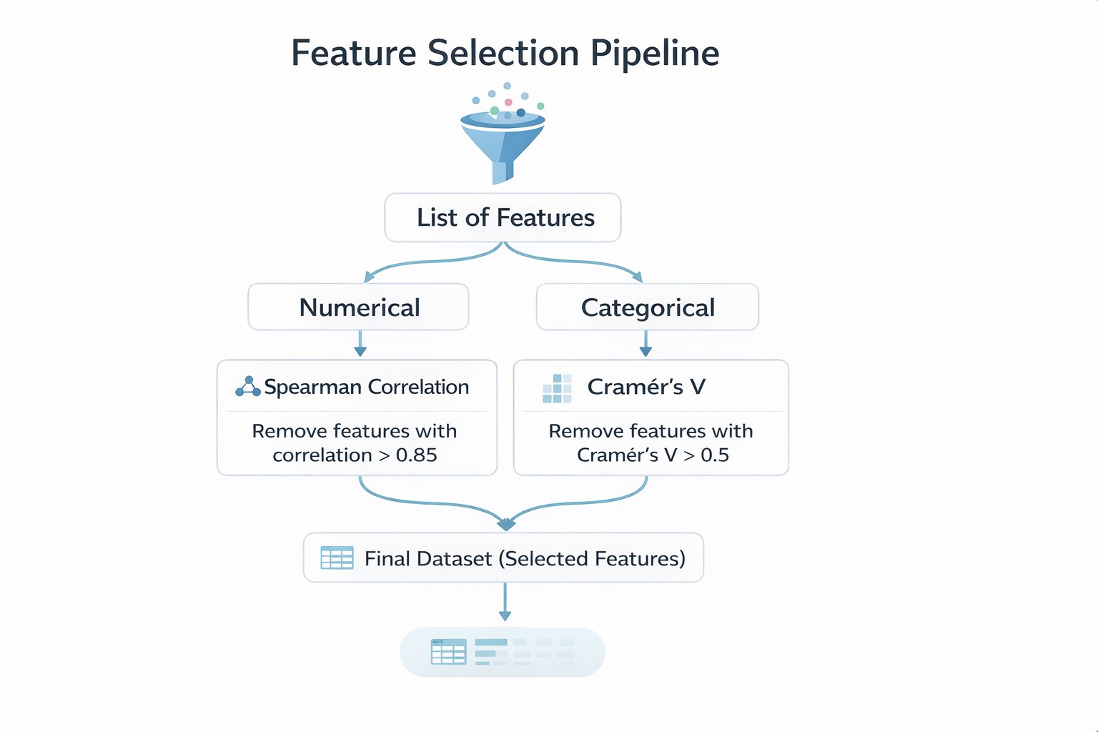
Graphical instruments are generally used to evaluate the discriminatory energy of variables. They’ll additionally assist consider the relationships between explanatory variables. This evaluation goals to scale back the variety of variables by figuring out those who present redundant data.

It’s usually carried out on variables of the identical sort—steady variables with steady variables, or categorical variables with categorical variables—since particular measures are designed for every case. For instance, we are able to use Spearman correlation for steady variables, or Cramér’s V and Tschuprow’s T for categorical variables to quantify the power of affiliation.

Within the following part, we assume that the accessible variables are related for discriminating default. It due to this fact turns into applicable to make use of statistical exams to additional examine the relationships between variables. We are going to describe a structured methodology for choosing the suitable exams and supply clear justification for these selections.

The objective is to not cowl each doable take a look at, however slightly to current a coherent and sturdy method that may information you in constructing a dependable scoring mannequin.

1.2 Multicollinearity Between Variables

In credit score scoring, once we discuss multicollinearity, the very first thing that normally involves thoughts is the Variance Inflation Issue (VIF). Nonetheless, there’s a a lot less complicated method that can be utilized when coping with numerous explanatory variables. This method permits for an preliminary screening of related variables and helps scale back dimensionality by analyzing the relationships between variables of the identical sort.

Within the following sections, we present how finding out the relationships between steady variables and between categorical variables might help determine redundant data and assist the preselection of explanatory variables.

1.2.1 Check statistic for the examine: Relationship Between Steady Explanatory Variables

In scoring fashions, analyzing the connection between two steady variables is usually used to pre-select variables and scale back dimensionality. This evaluation turns into notably related when the variety of explanatory variables could be very giant (e.g., greater than 100), as it could possibly considerably scale back the variety of variables.

On this part, we deal with the case of two steady explanatory variables. Within the subsequent part, we are going to look at the case of two categorical variables.

To check this affiliation, the Pearson correlation can be utilized. Nonetheless, usually, the Spearman correlation is most well-liked, as it’s a non-parametric measure. In distinction, Pearson correlation solely captures linear relationships between variables.

Spearman correlation is commonly most well-liked in follow as a result of it’s sturdy to outliers and doesn’t depend on distributional assumptions. It measures how nicely the connection between two variables will be described by a monotonic perform, whether or not linear or not.

Mathematically, it’s computed by making use of the Pearson correlation formulation to the ranked variables:

$rho_{X,Y} = frac{mathrm{Cov}(mathrm{Rank}_X, mathrm{Rank}_Y)}{sigma_{mathrm{Rank}_X} , sigma_{mathrm{Rank}_Y}}$

Due to this fact, on this context, Spearman correlation is chosen to evaluate the connection between two steady variables.

If two or extra unbiased steady variables exhibit a excessive pairwise Spearman correlation (e.g., ≥ 0.6 or 60%), this implies that they carry comparable data. In such instances, it’s applicable to retain solely considered one of them—both the variable that’s most strongly correlated with the goal (default) or the one thought of most related based mostly on area experience.

1.2.2 Check statistic for the examine: Relationship Between Qualitative Explanatory Variables.

As within the evaluation of the connection between an explanatory variable and the goal (default), Cramér’s V is used right here to evaluate whether or not two or extra qualitative variables present the identical data.

For instance, if Cramér’s V exceeds 0.5 (50%), the variables are thought of to be extremely related and should seize comparable data. Due to this fact, they shouldn’t be included concurrently within the mannequin, as this could introduce redundancy.

The selection of which variable to retain will be based mostly on statistical standards—equivalent to holding the variable that’s most strongly related to the goal (default)—or on area experience, by deciding on the variable thought of essentially the most related from a enterprise perspective.

As you could have observed, we examine the connection between a steady variable and a categorical variable as a part of the dimensionality discount course of, since there isn’t a direct indicator to measure the power of the affiliation, in contrast to Spearman correlation or Cramér’s V.

For these , one doable method is to make use of the Variance Inflation Issue (VIF). We are going to cowl this in a future publication. It’s not mentioned right here as a result of the methodology for computing VIF might differ relying on whether or not you utilize Python or R. These particular points can be addressed within the subsequent submit.

Within the following part, we are going to apply all the pieces mentioned to this point to real-world knowledge, particularly the dataset launched in our earlier article.

1.3 Software in the actual knowledge

This part analyzes the correlations between variables and contributes to the pre-selection of variables. The info used are these from the earlier article, the place outliers and lacking values have been already handled.

Three forms of correlations (every utilizing a special statistical take a look at seen above) are analyzed :

• Correlation between steady variables and the default variable (Kruskall-Wallis take a look at)
• Correlations between qualitatives variables and the default variables (Cramer’s V).
• Multi-correlations between steady variables (Spearman take a look at)
• Multi-correlations between qualitatives variables (Cramer’s V)

1.3.1 Correlation between steady variables and the default variable

Within the practice database, we’ve got seven steady variables :

• person_income
• person_age
• person_emp_length
• loan_amnt
• loan_int_rate
• loan_percent_income

The desk under presents the p-values from the Kruskal–Wallis take a look at, which measure the connection between these variables and the default variable.

def correlation_quanti_def_KW(database: pd.DataFrame,
                              continuous_vars: checklist,
                              goal: str) -> pd.DataFrame:
    """
    Compute Kruskal-Wallis take a look at p-values between steady variables
    and a categorical (binary or multi-class) goal.

    Parameters
    ----------
    database : pd.DataFrame
        Enter dataset
    continuous_vars : checklist
        Checklist of steady variable names
    goal : str
        Goal variable identify (categorical)

    Returns
    -------
    pd.DataFrame
        Desk with variables and corresponding p-values
    """

    outcomes = []

    for var in continuous_vars:
        # Drop NA for present variable + goal
        df = database[[var, target]].dropna()

        # Group values by goal classes
        teams = [
            group[var].values
            for _, group in df.groupby(goal)
        ]

        # Kruskal-Wallis requires a minimum of 2 teams
        if len(teams) < 2:
            p_value = None
        else:
            attempt:
                stat, p_value = kruskal(*teams)
            besides ValueError:
                # Handles edge instances (e.g., fixed values)
                p_value = None

        outcomes.append({
            "variable": var,
            "p_value": p_value,
            "stats_kw": stat if 'stat' in locals() else None
        })
       
    return pd.DataFrame(outcomes).sort_values(by="p_value")

continuous_vars = [
    "person_income",
    "person_age",
    "person_emp_length",
    "loan_amnt",
    "loan_int_rate",
    "loan_percent_income",
    "cb_person_cred_hist_length"
]
goal = "def"
consequence = correlation_quanti_def_KW(
    database=train_imputed,
    continuous_vars=continuous_vars,
    goal=goal
)

print(consequence)

# Save outcomes to xlsx
consequence.to_excel(f"{data_output_path}/correlation/correlations_kw.xlsx", index=False)

By evaluating the p-values to the 5% significance degree, we observe that each one are under the edge. Due to this fact, we reject the null speculation for all variables and conclude that every steady variable is considerably related to the default variable.

1.3.2 Correlations between qualitative variables and the default variables (Cramer’s V).

Within the database, we’ve got 4 qualitative variables :

• person_home_ownership
• cb_person_default_on_file
• loan_intent
• loan_grade

The desk under studies the power of the affiliation between these categorical variables and the default variable, as measured by Cramér’s V.

def cramers_v_with_target(database: pd.DataFrame,
                          categorical_vars: checklist,
                          goal: str) -> pd.DataFrame:
    """
    Compute Chi-square statistic and Cramér's V between a number of
    categorical variables and a goal variable.

    Parameters
    ----------
    database : pd.DataFrame
        Enter dataset
    categorical_vars : checklist
        Checklist of categorical variables
    goal : str
        Goal variable (categorical)

    Returns
    -------
    pd.DataFrame
        Desk with variable, chi2 and Cramér's V
    """

    outcomes = []

    for var in categorical_vars:
        # Drop lacking values
        df = database[[var, target]].dropna()

        # Contingency desk
        contingency_table = pd.crosstab(df[var], df[target])

        # Skip if not sufficient knowledge
        if contingency_table.form[0] < 2 or contingency_table.form[1] < 2:
            outcomes.append({
                "variable": var,
                "chi2": None,
                "cramers_v": None
            })
            proceed

        attempt:
            chi2, _, _, _ = chi2_contingency(contingency_table)
            n = contingency_table.values.sum()
            r, ok = contingency_table.form

            v = np.sqrt((chi2 / n) / min(ok - 1, r - 1))

        besides Exception:
            chi2, v = None, None

        outcomes.append({
            "variable": var,
            "chi2": chi2,
            "cramers_v": v
        })

    result_df = pd.DataFrame(outcomes)

    # Choice : tri par significance
    return result_df.sort_values(by="cramers_v", ascending=False)

qualitative_vars = [
    "person_home_ownership",
    "cb_person_default_on_file",
    "loan_intent",
    "loan_grade",
]
consequence = cramers_v_with_target(
    database=train_imputed,
    categorical_vars=qualitative_vars,
    goal=goal
)

print(consequence)

# Save outcomes to xlsx
consequence.to_excel(f"{data_output_path}/correlation/cramers_v.xlsx", index=False)

The outcomes point out that almost all variables are related to the default variable. A average affiliation is noticed for loan_grade, whereas the opposite categorical variables exhibit weak associations.

1.3.3 Multi-correlations between steady variables (Spearman take a look at)

To determine steady variables that present comparable data, we use the Spearman correlation with a threshold of 60%. That’s, if two steady explanatory variables exhibit a Spearman correlation above 60%, they’re thought of redundant and to seize comparable data.

def correlation_matrix_quanti(database: pd.DataFrame,
                              continuous_vars: checklist,
                              methodology: str = "spearman",
                              as_percent: bool = False) -> pd.DataFrame:
    """
    Compute correlation matrix for steady variables.

    Parameters
    ----------
    database : pd.DataFrame
        Enter dataset
    continuous_vars : checklist
        Checklist of steady variables
    methodology : str
        Correlation methodology ("pearson" or "spearman"), default = "spearman"
    as_percent : bool
        If True, return values in proportion

    Returns
    -------
    pd.DataFrame
        Correlation matrix
    """

    # Choose related knowledge and drop rows with NA
    df = database[continuous_vars].dropna()

    # Compute correlation matrix
    corr_matrix = df.corr(methodology=methodology)

    # Convert to proportion if required
    if as_percent:
        corr_matrix = corr_matrix * 100

    return corr_matrix

corr = correlation_matrix_quanti(
    database=train_imputed,
    continuous_vars=continuous_vars,
    methodology="spearman"
)

print(corr)

# Save outcomes to xlsx
corr.to_excel(f"{data_output_path}/correlation/correlation_matrix_spearman.xlsx")

We determine two pairs of variables which might be extremely correlated:

• The pair (cb_person_cred_hist_length, person_age) with a correlation of 85%
• The pair (loan_percent_income, loan_amnt) with a excessive correlation

Just one variable from every pair ought to be retained for modeling. We depend on statistical standards to pick out the variable that’s most strongly related to the default variable. On this case, we retain person_age and loan_percent_income.

1.3.4 Multi-correlations between qualitative variables (Cramer’s V)

On this part, we analyze the relationships between categorical variables. If two categorical variables are related to a Cramér’s V larger than 60%, considered one of them ought to be faraway from the candidate danger driver checklist to keep away from introducing extremely correlated variables into the mannequin.

The selection between the 2 variables will be based mostly on professional judgment. Nonetheless, on this case, we depend on a statistical method and choose the variable that’s most strongly related to the default variable.

The desk under presents the Cramér’s V matrix computed for every pair of categorical explanatory variables.

def cramers_v_matrix(database: pd.DataFrame,
                     categorical_vars: checklist,
                     corrected: bool = False,
                     as_percent: bool = False) -> pd.DataFrame:
    """
    Compute Cramér's V correlation matrix for categorical variables.

    Parameters
    ----------
    database : pd.DataFrame
        Enter dataset
    categorical_vars : checklist
        Checklist of categorical variables
    corrected : bool
        Apply bias correction (beneficial)
    as_percent : bool
        Return values in proportion

    Returns
    -------
    pd.DataFrame
        Cramér's V matrix
    """

    def cramers_v(x, y):
        # Drop NA
        df = pd.DataFrame({"x": x, "y": y}).dropna()

        contingency_table = pd.crosstab(df["x"], df["y"])

        if contingency_table.form[0] < 2 or contingency_table.form[1] < 2:
            return np.nan

        chi2, _, _, _ = chi2_contingency(contingency_table)
        n = contingency_table.values.sum()
        r, ok = contingency_table.form

        phi2 = chi2 / n

        if corrected:
            # Bergsma correction
            phi2_corr = max(0, phi2 - ((k-1)*(r-1)) / (n-1))
            r_corr = r - ((r-1)**2) / (n-1)
            k_corr = ok - ((k-1)**2) / (n-1)
            denom = min(k_corr - 1, r_corr - 1)
        else:
            denom = min(ok - 1, r - 1)

        if denom <= 0:
            return np.nan

        return np.sqrt(phi2_corr / denom) if corrected else np.sqrt(phi2 / denom)

    # Initialize matrix
    n = len(categorical_vars)
    matrix = pd.DataFrame(np.zeros((n, n)),
                          index=categorical_vars,
                          columns=categorical_vars)

    # Fill matrix
    for i, var1 in enumerate(categorical_vars):
        for j, var2 in enumerate(categorical_vars):
            if i <= j:
                worth = cramers_v(database[var1], database[var2])
                matrix.loc[var1, var2] = worth
                matrix.loc[var2, var1] = worth

    # Convert to proportion
    if as_percent:
        matrix = matrix * 100

    return matrix
matrix = cramers_v_matrix(
    database=train_imputed,
    categorical_vars=qualitative_vars,
)

print(matrix)
# Save outcomes to xlsx
matrix.to_excel(f"{data_output_path}/correlation/cramers_v_matrix.xlsx")

From this desk, utilizing a 60% threshold, we observe that just one pair of variables is strongly related: (loan_grade, cb_person_default_on_file). The variable we retain is loan_grade, as it’s extra strongly related to the default variable.

Primarily based on these analyses, we’ve got pre-selected 9 variables for the following steps. Two variables have been eliminated throughout the evaluation of correlations between steady variables, and one variable was eliminated throughout the evaluation of correlations between categorical variables.

Conclusion

The target of this submit was to current learn how to measure the totally different relationships that exist between variables in a credit score scoring mannequin.

We’ve seen that this evaluation can be utilized to guage the discriminatory energy of explanatory variables, that’s, their capacity to foretell the default variable. When the explanatory variable is steady, we are able to depend on the non-parametric Kruskal–Wallis take a look at to evaluate the connection between the variable and default.

When the explanatory variable is categorical, we use Cramér’s V, which measures the power of the affiliation and is much less delicate to pattern dimension than the chi-square take a look at alone.

Lastly, we’ve got proven that analyzing relationships between variables additionally helps scale back dimensionality by figuring out multicollinearity, particularly when variables are of the identical sort.

For 2 steady explanatory variables, we are able to use the Spearman correlation, with a threshold (e.g., 60%). If the Spearman correlation exceeds this threshold, the 2 variables are thought of redundant and shouldn’t each be included within the mannequin. One can then be chosen based mostly on its relationship with the default variable or based mostly on area experience.

For 2 categorical explanatory variables, we once more use Cramér’s V. By setting a threshold (e.g., 50%), we are able to assume that if Cramér’s V exceeds this worth, the variables present comparable data. On this case, solely one of many two variables ought to be retained—both based mostly on its discriminatory energy or by professional judgment.

In follow, we utilized these strategies to the dataset processed in our earlier submit. Whereas this method is efficient, it isn’t essentially the most sturdy methodology for variable choice. In our subsequent submit, we are going to current a extra sturdy method for pre-selecting variables in a scoring mannequin.

Picture Credit

All pictures and visualizations on this article have been created by the writer utilizing Python (pandas, matplotlib, seaborn, and plotly) and excel, until in any other case acknowledged.

References

[1] Lorenzo Beretta and Alessandro Santaniello.
Nearest Neighbor Imputation Algorithms: A Vital Analysis.
Nationwide Library of Drugs, 2016.

[2] Nexialog Consulting.
Traitement des données manquantes dans le milieu bancaire.
Working paper, 2022.

[3] John T. Hancock and Taghi M. Khoshgoftaar.
Survey on Categorical Knowledge for Neural Networks.
Journal of Huge Knowledge, 7(28), 2020.

[4] Melissa J. Azur, Elizabeth A. Stuart, Constantine Frangakis, and Philip J. Leaf.
A number of Imputation by Chained Equations: What Is It and How Does It Work?
Worldwide Journal of Strategies in Psychiatric Analysis, 2011.

[5] Majid Sarmad.
Sturdy Knowledge Evaluation for Factorial Experimental Designs: Improved Strategies and Software program.
Division of Mathematical Sciences, College of Durham, England, 2006.

[6] Daniel J. Stekhoven and Peter Bühlmann.
MissForest—Non-Parametric Lacking Worth Imputation for Combined-Sort Knowledge.Bioinformatics, 2011.

[7] Supriyanto Wibisono, Anwar, and Amin.
Multivariate Climate Anomaly Detection Utilizing the DBSCAN Clustering Algorithm.
Journal of Physics: Convention Collection, 2021.

[8] Laborda, J., & Ryoo, S. (2021). Characteristic choice in a credit score scoring mannequin. Arithmetic, 9(7), 746.

Knowledge & Licensing

The dataset used on this article is licensed underneath the Inventive Commons Attribution 4.0 Worldwide (CC BY 4.0) license.

This license permits anybody to share and adapt the dataset for any objective, together with industrial use, supplied that correct attribution is given to the supply.

For extra particulars, see the official license textual content: CC0: Public Area.

Disclaimer

Any remaining errors or inaccuracies are the writer’s accountability. Suggestions and corrections are welcome.