Achieve a Higher Understanding of Pc Imaginative and prescient: Dynamic SOLO (SOLOv2) with TensorFlow

https://github.com/syrax90/dynamic-solov2-tensorflow2 – Supply code of the challenge described within the article.

Disclaimer

⚠️ Initially, observe that this challenge shouldn’t be production-ready code.

and Why I Determined to Implement It from Scratch

This challenge targets individuals who don’t have high-performance {hardware} (GPU significantly) however need to examine laptop imaginative and prescient or at the least on the way in which of discovering themselves as an individual on this space. I attempted to make the code as clear as doable, so I used Google’s description fashion for all strategies and courses, feedback contained in the code to make the logic and calculations extra clear and used Single Accountability Precept and different OOP ideas to make the code extra human-readable.

Because the title of the article suggests, I made a decision to implement Dynamic SOLO from scratch to deeply perceive all of the intricacies of implementing such fashions, together with your entire cycle of practical manufacturing, to higher perceive the issues that may be encountered in laptop imaginative and prescient duties, and to realize useful expertise in creating laptop imaginative and prescient fashions utilizing TensorFlow. Wanting forward, I’ll say that I used to be not mistaken with this alternative, because it introduced me plenty of new abilities and information.

I’d suggest implementing fashions from scratch to everybody who need to perceive their ideas of working deeper. That’s why:

• If you encounter a misunderstanding about one thing, you begin to delve deeper into the precise downside. By exploring the issue, you discover a solution to the query of why a selected method was invented, and thus develop your information on this space.
• If you perceive the speculation behind an method or precept, you begin to discover find out how to implement it utilizing present technical instruments. On this manner, you enhance your technical abilities for fixing particular issues.
• When implementing one thing from scratch, you higher perceive the worth of the hassle, time, and sources that may be spent on such duties. By evaluating them with comparable duties, you extra precisely estimate the prices and have a greater thought of the worth of comparable work, together with preparation, analysis, technical implementation, and even documentation.

TensorFlow was chosen because the framework just because I exploit this framework for many of my machine studying duties (nothing particular right here).
The challenge represents implementation of Dynamic SOLO (SOLOv2) mannequin with TensorFlow2 framework.

SOLO: A Easy Framework for Occasion Segmentation,
Xinlong Wang, Rufeng Zhang, Chunhua Shen, Tao Kong, Lei Li
arXiv preprint (arXiv:2106.15947)

SOLO (Segmenting Objects by Areas) is a mannequin designed for laptop imaginative and prescient duties, specifically as an illustration segmentation. It’s completely anchor-free framework that predicts masks with none bounding containers. The paper presents a number of variants of the mannequin: Vanilla SOLO, Decoupled SOLO, Dynamic SOLO, Decoupled Dynamic SOLO. Certainly, I applied Vanilla SOLO first as a result of it’s the best of all of them. However I’m not going to publish the code as a result of there isn’t any giant distinguish between Vanilla and Dynamic SOLO from implementation viewpoint.

Mannequin

Truly, the mannequin might be very versatile in accordance with the ideas described within the SOLO paper: from the variety of FPN layers to the variety of parameters within the layers. I made a decision to begin with the only implementation. The fundamental thought of the mannequin is to divide your entire picture into cells, the place one grid cell can signify just one occasion: decided class + segmentation masks.

Spine

I selected ResNet50 because the spine as a result of it’s a light-weight community that fits for starting completely. I didn’t use pretrained parameters for ResNet50 as a result of I used to be experimenting with extra than simply unique COCO dataset. Nonetheless, you need to use pretrained parameters should you intend to make use of the unique COCO dataset, because it saves time, accelerates the coaching course of, and improves efficiency.

spine = ResNet50(weights='imagenet', include_top=False, input_shape=input_shape)
spine.trainable = False

Neck

FPN (Characteristic Pyramid Community) is used because the neck for extracting multi-scale options. Throughout the FPN, we use all outputs C2, C3, C4, C5 from the corresponding residual blocks of ResNet50 as described within the FPN paper (Characteristic Pyramid Networks for Object Detection by Tsung-Yi Lin, Piotr Dollár, Ross Girshick, Kaiming He, Bharath Hariharan, Serge Belongie). Every FPN stage represents a particular scale and has its personal grid as proven above.

Notice: You shouldn’t use all FPN ranges should you work with a small customized dataset the place all objects are roughly the identical scale. In any other case, you prepare further parameters that aren’t used and consequently require extra GPU sources in useless. In that case, you’d have to regulate the dataset in order that it returns targets for simply 1 scale, not all 4.

Head

The outputs of the FPN layers are used as inputs to layers the place the occasion class and its masks are decided. Head accommodates two parallel branches for the intention: Classification department and Masks kernel department.

Notice: I excluded Masks Characteristic from the Head based mostly on the Vanilla Head structure. Masks Characteristic is described individually beneath.

• Classification department (within the determine above it’s designated as “Class”) – is chargeable for predicting the category of every occasion (grid cell) in a picture. It consists of a sequence of Conv2D -> GroupNorm -> ReLU units organized in a row. I utilized a sequence of 4 such units.
• Masks department (within the determine above it’s designated as “Masks”) – here’s a essential nuance: in contrast to within the Vanilla SOLO mannequin, it doesn’t generate masks immediately. As a substitute, it predicts a masks kernel (known as “Masks kernel” in Part 3.2.3 Dynamic SOLO of the paper), which is later utilized via dynamic convolution with the Masks characteristic described beneath. This design differentiates Dynamic SOLO from Vanilla SOLO by lowering the variety of parameters and making a extra environment friendly, light-weight structure. The Masks department predicts a masks kernel for every occasion (grid cell) utilizing the identical construction because the Classification department: a sequence of Conv2D -> GroupNorm -> ReLU units organized in a row. I additionally applied 4 such units within the mannequin.

Notice: For small customized datasets, you possibly can usen even 1 such set for each the masks and classification branches, avoiding coaching pointless parameters

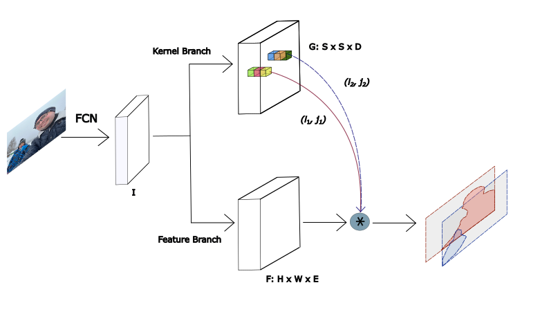
Masks Characteristic

The Masks characteristic department is mixed with the Masks kernel department to find out the ultimate predicted masks. This layer fuses multi-level FPN options to supply a unified masks characteristic map. The authors of the paper evaluated two approaches to implementing the Masks characteristic department: a particular masks characteristic for every FPN stage or one unified masks characteristic for all FPN ranges. Just like the authors, I selected the final one. The Masks characteristic department and Masks kernel department are mixed by way of dynamic convolution operation.

Dataset

I selected to work with the COCO dataset format, coaching my mannequin on each the unique COCO dataset and a small customized dataset structured in the identical format. I selected COCO format as a result of it has already been broadly researched, that makes writing code for parsing the format a lot simpler. Furthermore, the LabelMe device I selected to construct my customized dataset in a position to convert a dataset on to COCO format. Moreover, beginning with a small customized dataset reduces coaching time and simplifies the event course of. Another reason to create a dataset by your self is the chance to higher perceive the dataset creation course of, take part in it immediately, and achieve new abilities in interacting with instruments like LabelMe. A small annotation file might be explored sooner and simpler than a big file if you wish to dive deeper into the COCO format.

Listed below are a number of the sub-tasks concerning datasets that I encountered whereas implementing the challenge (they’re offered within the challenge):

• Information augmentation. Information augmentation of a picture dataset is the method of increasing the dataset by making use of varied picture transformation strategies to generate new samples that differ from the unique ones. Mastering augmentation strategies is crucial, particularly for small datasets. I utilized strategies comparable to Horizontal flip, Brightness adjustment, Random scaling, Random cropping to present an thought of how to do that and perceive how necessary it’s that the masks of the modified picture matches its new (augmented) picture.
• Changing to focus on. The SOLO mannequin expects a particular information format for the goal. It takes a normalized picture as enter, nothing particular. However for the goal, the mannequin expects extra advanced information:
  • We now have to construct a grid for every scale separating it by the variety of grid cells for the precise scale. That signifies that if we’ve 4 FPN ranges – P2, P3, P4, P5 – for various scales, then we could have 4 grids with a sure variety of cells for every scale.
  • For every occasion, we’ve to outline by location the one cell to which the occasion belongs amongst all of the grids.
  • For every outlined, the class and masks of the corresponding occasion are utilized. There may be an extra downside of changing the COCO format masks right into a masks consisting of ones for the masks pixels and zeros for the remainder of the pixels.
  • Mix all the above into a listing of tensors because the goal. I perceive that TensorFlow prefers a strict set of tensors over constructions like a listing, however I made a decision to decide on a listing for the added flexibility that you just may want should you determine to alter the variety of scales.
• Dataset in reminiscence or Generated. The are two predominant choices for dataset allocation: storing samples in reminiscence or producing information on the fly. Regardless of of allocation in reminiscence has plenty of benefits and there’s no downside for lots of you to add total coaching dataset listing of COCO dataset into reminiscence (19.3 GB solely) – I deliberately selected to generate the dataset dynamically utilizing tf.information.Dataset.from_generator. Right here’s why: I believe it’s ability to be taught what issues you may encounter interacting with massive information and find out how to resolve them. As a result of when working with real-world issues, datasets could not solely comprise extra samples than COCO datasets, however their decision can also be a lot increased. Working with dynamically generated datasets is mostly a bit extra advanced to implement, however it’s extra versatile. After all, you possibly can change it with tf.information.Dataset.from_tensor_slices, if you want.

Coaching Course of

Loss Operate

SOLO doesn’t have a typical Loss Operate that isn’t natively applied in TensorFlow, so I applied it on my own.

$$L = L_{cate} + lambda L_{masks}$$

The place:

• (L_{cate}) is the standard Focal Loss for semantic class classification.
• (L_{masks}) is the loss for masks prediction.
• (lambda) coefficient that’s set to three within the paper.

$$
L_{masks}
=
frac{1}{N_{pos}}
sum_k
mathbb{1}_{{p^*_{i,j} > 0}}
d_{masks}(m_k, m^*_k)
$$

The place:

• (N_{pos}) is the variety of optimistic samples.
• (d_{masks}) is applied as Cube Loss.
• ( i = lfloor okay/S rfloor ), ( j = okay mod S ) — Indices for grid cells, indexing left to proper and high to backside.
• 1 is the indicator operate, being 1 if (p^*_{i,j} > 0) and 0 in any other case.

$$L_{Cube}=1 – D(p, q)$$

The place D is the cube coefficient, which is outlined as

$$
D(p, q)
=
frac
{2 sum_{x,y} (p_{x,y} cdot q_{x,y})}
{sum_{x,y} p^2_{x,y} + sum_{x,y} q^2_{x,y}}
$$

The place (p_{x,y}), (q_{x,y}) are pixel values at (x,y) for predicted masks p and floor fact masks q. All particulars of the loss operate are described in 3.3.2 Loss Operate of the unique SOLO paper

Resuming from Checkpoint.

Should you use a low-performance GPU, you may encounter conditions the place coaching your entire mannequin in a single run is impractical. So as to not lose your educated weights and proceed to execute the coaching course of – this challenge gives a Resuming from Checkpoint system. It lets you save your mannequin each n epochs (the place n is configurable) and resume coaching later. To allow this, set load_previous_model to True and specify model_path in config.py.

self.load_previous_model = True
self.model_path = './weights/coco_epoch00000001.keras'

Analysis Course of

To see how successfully your mannequin is educated and the way nicely it behaves on beforehand unseen photographs, an analysis course of is used. For the SOLO mannequin, I’d break down the method into the next steps:

1. Loading a check dataset.
2. Making ready the dataset to be appropriate for the mannequin’s enter.
3. Feeding the information into the mannequin.
4. Suppressing ensuing masks with decrease chance for a similar occasion.
5. Visualization of the unique check picture with the ultimate masks and predicted class for every occasion.

Essentially the most irregular job I confronted right here was implementing Matrix NMS (non-maximum suppression), described in 3.3.4 Matrix NMS of the unique SOLO paper. NMS eliminates redundant masks representing the identical occasion with decrease chance. To keep away from predicting the identical occasion a number of instances, we have to suppress these duplicate masks. The authors supplied Python pseudo-code for Matrix NMS and certainly one of my duties was to interpret this pseudo-code and implement it utilizing TensorFlow. My implementation:

def matrix_nms(masks, scores, labels, pre_nms_k=500, post_nms_k=100, score_threshold=0.5, sigma=0.5):
    """
    Carry out class-wise Matrix NMS on occasion masks.

    Parameters:
        masks (tf.Tensor): Tensor of form (N, H, W) with every masks as a sigmoid chance map (0~1).
        scores (tf.Tensor): Tensor of form (N,) with confidence scores for every masks.
        labels (tf.Tensor): Tensor of form (N,) with class labels for every masks (ints).
        pre_nms_k (int): Variety of top-scoring masks to maintain earlier than making use of NMS.
        post_nms_k (int): Variety of closing masks to maintain after NMS.
        score_threshold (float): Rating threshold to filter out masks after NMS (default 0.5).
        sigma (float): Sigma worth for Gaussian decay.

    Returns:
        tf.Tensor: Tensor of indices of masks saved after suppression.
    """
    # Binarize masks at 0.5 threshold
    seg_masks = tf.solid(masks >= 0.5, dtype=tf.float32)  # form: (N, H, W)
    mask_sum = tf.reduce_sum(seg_masks, axis=[1, 2])  # form: (N,)

    # If desired, choose high pre_nms_k by rating to restrict computation
    num_masks = tf.form(scores)[0]
    if pre_nms_k shouldn't be None:
        num_selected = tf.minimal(pre_nms_k, num_masks)
    else:
        num_selected = num_masks
    topk_indices = tf.argsort(scores, course='DESCENDING')[:num_selected]
    seg_masks = tf.collect(seg_masks, topk_indices)  # choose masks by high scores
    labels_sel = tf.collect(labels, topk_indices)
    scores_sel = tf.collect(scores, topk_indices)
    mask_sum_sel = tf.collect(mask_sum, topk_indices)

    # Flatten masks for matrix operations
    N = tf.form(seg_masks)[0]
    seg_masks_flat = tf.reshape(seg_masks, (N, -1))  # form: (N, H*W)

    # Compute intersection and IoU matrix (N x N)
    intersection = tf.matmul(seg_masks_flat, seg_masks_flat, transpose_b=True)  # pairwise intersect counts
    # Broaden masks areas to full matrices
    mask_sum_matrix = tf.tile(mask_sum_sel[tf.newaxis, :], [N, 1])  # form: (N, N)
    union = mask_sum_matrix + tf.transpose(mask_sum_matrix) - intersection
    iou = intersection / (union + 1e-6)  # IoU matrix (keep away from div-by-zero)
    # Zero out diagonal and decrease triangle (hold i= score_threshold                        # boolean mask of those above threshold
    new_scores = tf.where(keep_mask, new_scores, tf.zeros_like(new_scores))

    # Select top post_nms_k by the decayed scores
    if post_nms_k is not None:
        num_final = tf.minimum(post_nms_k, tf.shape(new_scores)[0])
    else:
        num_final = tf.form(new_scores)[0]
    final_indices = tf.argsort(new_scores, course='DESCENDING')[:num_final]
    final_indices = tf.boolean_mask(final_indices, tf.larger(tf.collect(new_scores, final_indices), 0))

    # Map again to unique indices
    kept_indices = tf.collect(topk_indices, final_indices)
    return kept_indices

Beneath is an instance of photographs with overlaid masks predicted by the mannequin for a picture it has by no means seen earlier than:

Recommendation for Implementation from Scratch

• Which information will we map to which operate? It is rather necessary to be sure that we feed the best information to the mannequin. The information ought to match what is predicted at every layer, and every layer processes the enter information in order that the output is appropriate for the following layer. As a result of we finally calculate the loss operate based mostly on this information. Based mostly on the implementation of SOLO, I noticed that some targets will not be so simple as they appear at first look. I described this within the Dataset chapter.
• Analysis the paper. It’s not possible to flee studying the paper you might be about to construct your mannequin based mostly on. I do know it’s apparent, however regardless of the various references to different earlier works and papers, it’s essential to perceive the ideas. If you begin researching a paper, it’s possible you’ll be confronted with plenty of different papers that it’s essential to learn and perceive earlier than you are able to do so, and this may be fairly a difficult job. However normally, even essentially the most up-to-date paper is predicated on a set of ideas which have been recognized for a while and will not be new. Because of this you will discover plenty of materials on the Web that describes these ideas very clearly. You need to use LLM packages for this objective, which might summarize the knowledge, give examples, and allow you to perceive a number of the works and papers.
• Begin with small steps. That is trivial recommendation, however to implement a pc imaginative and prescient mannequin with tens of millions of parameters, you don’t have to waste time on ineffective coaching, dataset preparation, analysis, and many others. if you’re within the improvement stage and will not be positive that the mannequin will work accurately. Furthermore, when you’ve got a low-performance GPU, the method takes even longer. So, don’t begin with big datasets, many parameters, and a sequence of layers. You possibly can even let the mannequin overfit within the first stage of improvement with a small dataset and a small variety of parameters, to ensure that the information is accurately matched to the targets of the mannequin.
• Debug your code. Debugging your code lets you ensure that you could have anticipated code behaviour and information worth on every step. I perceive that everybody who at the least as soon as developed a software program product is aware of about it, and so they don’t want the recommendation. However I wish to spotlight it anyway as a result of constructing fashions, writing Loss Operate, making ready datasets for enter and targets we work together with math operations and tensors rather a lot. And it requires elevated consideration from us in contrast to routine programming code we face on a regular basis and know the way it works with out debugging.

Conclusion

This can be a transient description of the challenge with none technical particulars, to present a basic image and keep away from studying fatigue. Clearly, an outline of a challenge devoted to a pc imaginative and prescient mannequin can’t be slot in one article. If I see curiosity within the challenge from readers, I could write a extra detailed evaluation with technical particulars.

Thanks for studying!