


In my earlier submit I appeared on the affect of various hyperparameters on resolution bushes, each their efficiency and the way they seem visually.
The pure subsequent step, then, is random forests, utilizing sklearn.ensemble.RandomForestRegressor.
Once more, I received’t go into how the random forests work, areas resembling bootstrapping and have choice and majority voting. Basically, a random forest is a large variety of bushes working collectively (therefore a forest), and that’s all we care about.
I’ll use the identical information (California housing dataset through scikit-learn, CC-BY) and the identical normal course of, so in case you haven’t seen my earlier submit, I’d counsel studying that first, because it goes over a few of the capabilities and metrics I’m utilizing right here.
Code for that is in the identical repo as earlier than: https://github.com/jamesdeluk/data-projects/tree/essential/visualising-trees
As earlier than, all pictures beneath are created by me.
A primary forest
First, let’s see how a primary random forest performs, i.e. rf = RandomForestRegressor(random_state=42). The default mannequin has a vast max depth, and 100 bushes. Utilizing the average-of-ten methodology, it took ~6 seconds to suit and ~0.1 seconds to foretell – given it’s a forest and never a single tree, it’s not shocking it took 50 to 150 occasions longer than the deep resolution tree. And the scores?
| Metric | max_depth=None |
|---|---|
| MAE | 0.33 |
| MAPE | 0.19 |
| MSE | 0.26 |
| RMSE | 0.51 |
| R² | 0.80 |
It predicted 0.954 for my chosen row, in contrast with the precise worth of 0.894.
Sure, the out-of-the-box random forest carried out higher than the Bayes-search-tuned resolution tree from my earlier submit!
Visualising
There are just a few methods to visualise a random forest, such because the bushes, the predictions, and the errors. Function importances may also be used to match the person bushes in a forest.
Particular person tree plots
Pretty clearly, you may plot a person resolution tree. They are often accessed utilizing rf.estimators_. For instance, that is the primary one:

This one has a depth of 34, 9,432 leaves, and 18,863 nodes. And this random forest has 100 related bushes!
Particular person predictions
A method I wish to visualise random forests is plotting the person predictions for every tree. For instance, I can achieve this for my chosen row with [tree.predict(chosen[features].values) for tree in rf.estimators_], and plot the outcomes on a scatter:

As a reminder, the true worth is 0.894. You may simply see how, whereas some bushes had been means off, the imply of all of the predictions is fairly shut — much like the central restrict theorem (CLT). That is my favorite means of seeing the magic of random forests.
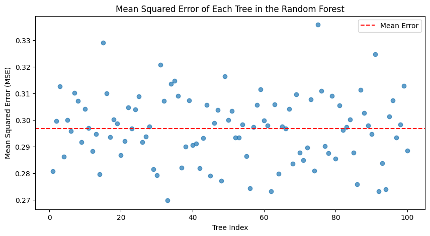
Particular person errors
Taking this one step additional, you may iterate by means of all of the bushes, have them make predictions for your entire dataset, then calculate an error statistic. On this case, for MSE:

The imply MSE was ~0.30, so barely greater than the general random forest — once more exhibiting the benefit of a forest over a single tree. The most effective tree was quantity 32, with an MSE of 0.27; the worst, 74, was 0.34 — though nonetheless fairly respectable. They each have depths of 34±1, with ~9400 leaves and ~18000 nodes — so, structurally, very related.
Function importances
Clearly a plot with all of the bushes can be tough to see, so that is the importances for the general forest, with the most effective and worst tree:

The most effective and worst bushes nonetheless have related importances for the completely different options — though the order is just not essentially the identical. Median revenue is by far an important issue based mostly on this evaluation.
Hyperparameter tuning
The identical hyperparameters that apply to particular person resolution bushes do, after all, apply to random forests made up of resolution bushes. For comparability’s sake, I created some RFs with the values I’d used within the earlier submit:
| Metric | max_depth=3 | ccp_alpha=0.005 | min_samples_split=10 | min_samples_leaf=10 | max_leaf_nodes=100 |
|---|---|---|---|---|---|
| Time to suit (s) | 1.43 | 25.04 | 3.84 | 3.77 | 3.32 |
| Time to foretell (s) | 0.006 | 0.013 | 0.028 | 0.029 | 0.020 |
| MAE | 0.58 | 0.49 | 0.37 | 0.37 | 0.41 |
| MAPE | 0.37 | 0.30 | 0.22 | 0.22 | 0.25 |
| MSE | 0.60 | 0.45 | 0.29 | 0.30 | 0.34 |
| RMSE | 0.78 | 0.67 | 0.54 | 0.55 | 0.58 |
| R² | 0.54 | 0.66 | 0.78 | 0.77 | 0.74 |
| Chosen prediction | 1.208 | 1.024 | 0.935 | 0.920 | 0.969 |
The very first thing we see — none carried out higher than the default tree (max_depth=None) above. That is completely different from the person resolution bushes, the place those with constraints carried out higher — once more demonstrating that the facility of a CLT-powered imperfect forest over one “good” tree. Nonetheless, much like earlier than, ccp_alpha takes a very long time, and shallow bushes are fairly garbage.
Past these, there are some hyperparameters that RFs have that DTs don’t. An important one is n_estimators — in different phrases, the variety of bushes!
n_jobs
However first, n_jobs. That is what number of jobs to run in parallel. Doing issues in parallel is often sooner than in serial/sequentially. The ensuing RF would be the similar, with the identical error and so forth scores (assuming random_state is about), nevertheless it must be completed faster! To check this, I added n_jobs=-1 to the default RF — on this context, -1 means “all”.
Bear in mind how the default one took nearly 6 seconds to suit and 0.1 to foretell? Parallelised, it took only one.1 seconds, and 0.03 to foretell — a 3~6x enchancment. I’ll undoubtedly be doing this to any extent further!
n_estimators
OK, again to the variety of bushes. The default RF has 100 estimators; let’s strive 1000. It took ~10 occasions as lengthy (9.7 seconds to suit, 0.3 to foretell, when parallelised), as one might need predicted. The scores?
| Metric | n_estimators=1000 |
|---|---|
| MAE | 0.328 |
| MAPE | 0.191 |
| MSE | 0.252 |
| RMSE | 0.502 |
| R² | 0.807 |
Little or no distinction; MSE and RMSE are 0.01 decrease, and R² is 0.01 greater. So higher, however well worth the 10x time funding?
Let’s cross-validate, simply to examine.
Moderately than use my customized loop, I’ll use sklearn.model_selection.cross_validate, as touched on within the earlier submit:
cross_validate(
    rf, X, y,
    cv=RepeatedKFold(n_splits=5, n_repeats=20, random_state=42),
    n_jobs=-1,
    scoring={
        "neg_mean_absolute_error": "neg_mean_absolute_error",
        "neg_mean_absolute_percentage_error": "neg_mean_absolute_percentage_error",
        "neg_mean_squared_error": "neg_mean_squared_error",
        "root_mean_squared_error": make_scorer(
            lambda y_true, y_pred: np.sqrt(mean_squared_error(y_true, y_pred)),
            greater_is_better=False,
        ),
        "r2": "r2",
    },
)
I’m utilizing RepeatedKFold because the splitting technique, which is extra secure however slower than KFold; because the dataset isn’t that large, I’m not too involved concerning the further time it would take.
As there is no such thing as a normal RMSE scorer, so I needed to create one with sklearn.metrics.make_scorer and a lambda operate.
For the choice bushes, I did 1000 loops. Nonetheless, given the default random forest incorporates 100 bushes, 1000 loops can be a lot of bushes, and due to this fact take a lot of time. I’ll strive 100 (20 repeats of 5 splits) — nonetheless loads, however due to parallelisation it wasn’t too dangerous — the 100 bushes model took 2mins (1304 seconds of unparallelised time), and the 1000 one took 18mins (10254s!) Nearly 100% CPU throughout all cores, and it bought fairly toasty — it’s not typically my MacBook followers activate, however this maxed them out!
How do they examine? The 100-tree one:
| Metric | Imply | Std |
|---|---|---|
| MAE | -0.328 | 0.006 |
| MAPE | -0.184 | 0.005 |
| MSE | -0.253 | 0.010 |
| RMSE | -0.503 | 0.009 |
| R² | 0.810 | 0.007 |
and the 1000-tree one:
| Metric | Imply | Std |
|---|---|---|
| MAE | -0.325 | 0.006 |
| MAPE | -0.183 | 0.005 |
| MSE | -0.250 | 0.010 |
| RMSE | -0.500 | 0.010 |
| R² | 0.812 | 0.006 |
Little or no distinction — in all probability not value the additional time/energy.
Bayes looking
Lastly, let’s do a Bayes search. I used a large hyperparameter vary.
search_spaces = {
    'n_estimators': (50, 500),
    'max_depth': (1, 100),
    'min_samples_split': (2, 100),
    'min_samples_leaf': (1, 100),
    'max_leaf_nodes': (2, 20000),
    'max_features': (0.1, 1.0, 'uniform'),
    'bootstrap': [True, False],
    'ccp_alpha': (0.0, 1.0, 'uniform'),
}
The one hyperparameter we haven’t seen to date is bootstrap; this determines whether or not to make use of the entire dataset when constructing a tree, or utilizing a bootstrap-based (pattern with substitute) strategy. Mostly that is set to True, however let’s strive False anyway.
I did 200 iterations, which took 66 (!!) minutes. It gave:
Greatest Parameters: OrderedDict({
    'bootstrap': False,
    'ccp_alpha': 0.0,
    'criterion': 'squared_error',
    'max_depth': 39,
    'max_features': 0.4863711682589259,
    'max_leaf_nodes': 20000,
    'min_samples_leaf': 1,
    'min_samples_split': 2,
    'n_estimators': 380
})
See how max_depth was much like the easy ones above, however n_estimators and max_leaf_nodes had been very excessive (notice max_leaf_nodes is just not the precise variety of leaf nodes, simply the utmost allowed worth; the imply variety of leaves was 14,954). min_samples_ had been each the minimal — much like earlier than once we in contrast the constrained forests to the unconstrained one. Additionally fascinating the way it didn’t bootstrap.
What does that give us (the short take a look at, not the cross validated one)?
| Metric | Worth |
|---|---|
| MAE | 0.313 |
| MAPE | 0.181 |
| MSE | 0.229 |
| RMSE | 0.478 |
| R² | 0.825 |
The most effective to date, though solely simply. For consistency, I additionally cross validated:
| Metric | Imply | Std |
|---|---|---|
| MAE | -0.309 | 0.005 |
| MAPE | -0.174 | 0.005 |
| MSE | -0.227 | 0.009 |
| RMSE | -0.476 | 0.010 |
| R² | 0.830 | 0.006 |
It’s performing very effectively. Evaluating absolutely the errors for the most effective resolution tree (the Bayes search one), the default RF, and the Bayes searched RF, offers us:

Conclusion
Within the final submit, the Bayes resolution tree appeared good, particularly in contrast with the essential resolution tree; now it appears horrible, with greater errors, decrease R², and wider variances! So why not all the time use a random forest?
Effectively, random forests do take loads longer to suit (and predict), and this turns into much more excessive with bigger datasets. Doing hundreds of tuning iterations on a forest with a whole lot of bushes and a dataset of tens of millions of rows and a whole lot of options… Even with parallelisation, it could actually take a very long time. It makes it fairly clear why GPUs, which concentrate on parallel processing, have turn out to be important for machine studying. Even so, you need to ask your self — what is nice sufficient? Does the ~0.05 enchancment in MAE truly matter to your use case?
On the subject of visualisation, as with resolution bushes, plotting particular person bushes is usually a good solution to get an concept of the general construction. Moreover, plotting the person predictions and errors is a good way to see the variance of a random forest, and get a greater understanding of how they work.
However there are extra tree variants! Subsequent, gradient boosted ones.


