


that 80% of knowledge collected, saved and maintained by governments will be related to geographical areas. Though by no means empirically confirmed, it illustrates the significance of location inside information. Ever rising information volumes put constraints on programs that deal with geospatial information. Frequent Massive Information compute engines, initially designed to scale for textual information, want adaptation to work effectively with geospatial information — consider geographical indexes, partitioning, and operators. Right here, I current and illustrate easy methods to make the most of the Microsoft Cloth Spark compute engine, with the natively built-in ESRI GeoAnalytics engine# for geospatial huge information processing and analytics.
The non-obligatory GeoAnalytics capabilities inside Cloth allow the processing and analytics of vector-type geospatial information, the place vector-type geospatial information refers to factors, traces, polygons. These capabilities embrace greater than 150 spatial capabilities to create geometries, take a look at, and choose spatial relationships. Because it extends Spark, the GeoAnalytics capabilities will be known as when utilizing Python, SQL, or Scala. These spatial operations apply routinely spatial indexing, making the Spark compute engine additionally environment friendly for this information. It may possibly deal with 10 additional frequent spatial information codecs to load and save information spatial information, on high of the Spark natively supported information supply codecs. This weblog submit focuses on the scalable geospatial compute engines as has been launched in my submit about geospatial within the age of AI.
Demonstration defined
Right here, I exhibit a few of these spatial capabilities by displaying the information manipulation and analytics steps on a big dataset. By utilizing a number of tiles overlaying level cloud information (a bunch of x, y, z values), an infinite dataset begins to kind, whereas it nonetheless covers a comparatively small space. The open Dutch AHN dataset, which is a nationwide digital elevation and floor mannequin, is at present in its fifth replace cycle, and spans a interval of almost 30 years. Right here, the information from the second, third, and forth acquisition is used, as these maintain full nationwide protection (the fifth simply not but), whereas the primary model didn’t embrace a degree cloud launch (solely the by-product gridded model).
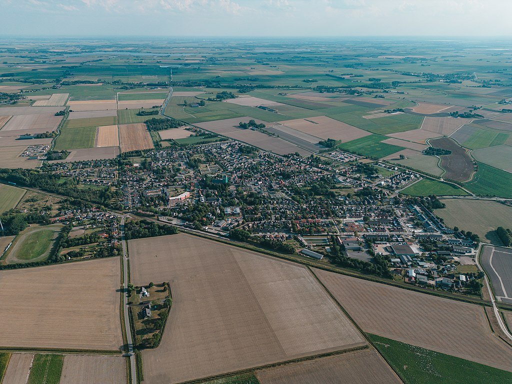
One other Dutch open dataset, particularly constructing information, the BAG, is used for example spatial choice. The constructing dataset incorporates the footprint of the buildings as polygons. At the moment, this dataset holds greater than 11 million buildings. To check the spatial capabilities, I take advantage of solely 4 AHN tiles per AHN model. Thus on this case, 12 tiles, every of 5 x 6.25 km. Totalling to greater than 3.5 billion factors inside an space of 125 sq. kilometers. The chosen space covers the municipality of Loppersum, an space liable to land subsidence as a result of fuel extraction.
The steps to take embrace the collection of buildings inside the space of Loppersum, choosing the x,y,z-points from the roofs of the buildings. Then, we carry the three datasets into one dataframe and do an additional evaluation with it. A spatial regression to foretell the anticipated peak of a constructing primarily based on its peak historical past in addition to the historical past of the buildings in its direct environment. Not essentially the perfect evaluation to carry out on this information to return to precise predictions* however it fits merely the aim of demonstrating the spatial processing capabilities of Cloth’s ESRI GeoAnalytics. All of the beneath code snippets are additionally accessible as notebooks on github.
Step 1: Learn information
Spatial information can are available in many various information codecs; we conform to the geoparquet information format for additional processing. The BAG constructing information, each the footprints in addition to the accompanied municipality boundaries, are available in geoparquet format already. The purpose cloud AHN information, model 2, 3 and 4, nonetheless, comes as LAZ file codecs — a compressed business commonplace format for level clouds. I’ve not discovered a Spark library to learn LAZ (please go away a message in case there may be one), and created a txt file, individually, with the LAStools+ first.
# ESRI - FABRIC reference: https://builders.arcgis.com/geoanalytics-fabric/

# Import the required modules
import geoanalytics_fabric
from geoanalytics_fabric.sql import capabilities as ST
from geoanalytics_fabric import extensions

# Learn ahn file from OneLake
# AHN lidar information supply: https://viewer.ahn.nl/

ahn_csv_path = "Information/AHN lidar/AHN4_csv"
lidar_df = spark.learn.choices(delimiter=" ").csv(ahn_csv_path)
lidar_df = lidar_df.selectExpr("_c0 as X", "_c1 as Y", "_c2 Z")

lidar_df.printSchema()
lidar_df.present(5)
lidar_df.depend()
The above code snippet& offers the beneath outcomes:

Now, with the spatial capabilities make_point and srid the x,y,z columns are remodeled to a degree geometry and set it to the precise Dutch coordinate system (SRID = 28992), see the beneath code snippet&:
# Create level geometry from x,y,z columns and set the spatial refrence system
lidar_df = lidar_df.choose(ST.make_point(x="X", y="Y", z="Z").alias("rd_point"))
lidar_df = lidar_df.withColumn("srid", ST.srid("rd_point"))
lidar_df = lidar_df.choose(ST.srid("rd_point", 28992).alias("rd_point"))
  .withColumn("srid", ST.srid("rd_point"))

lidar_df.printSchema()
lidar_df.present(5)

Constructing and municipality information will be learn with the prolonged spark.learn operate for geoparquet, see the code snippet&:
# Learn constructing polygon information
path_building = "Information/BAG NL/BAG_pand_202504.parquet"
df_buildings = spark.learn.format("geoparquet").load(path_building)

# Learn woonplaats information (=municipality)
path_woonplaats = "Information/BAG NL/BAG_woonplaats_202504.parquet"
df_woonplaats = spark.learn.format("geoparquet").load(path_woonplaats)

# Filter the DataFrame the place the "woonplaats" column incorporates the string "Loppersum"
df_loppersum = df_woonplaats.filter(col("woonplaats").incorporates("Loppersum"))
Step 2: Make alternatives
Within the accompanying notebooks, I learn and write to geoparquet. To verify the precise information is learn appropriately as dataframes, see the next code snippet:
# Learn constructing polygon information
path_building = "Information/BAG NL/BAG_pand_202504.parquet"
df_buildings = spark.learn.format("geoparquet").load(path_building)

# Learn woonplaats information (=municipality)
path_woonplaats = "Information/BAG NL/BAG_woonplaats_202504.parquet"
df_woonplaats = spark.learn.format("geoparquet").load(path_woonplaats)

# Filter the DataFrame the place the "woonplaats" column incorporates the string "Loppersum"
df_loppersum = df_woonplaats.filter(col("woonplaats").incorporates("Loppersum"))
With all information in dataframes it turns into a easy step to do spatial alternatives. The next code snippet& exhibits easy methods to choose the buildings inside the boundaries of the Loppersum municipality, and individually makes a collection of buildings that existed all through the interval (level cloud AHN-2 information was acquired in 2009 on this area). This resulted in 1196 buildings, out of the 2492 buildings at present.
# Clip the BAG buildings to the gemeente Loppersum boundary
df_buildings_roi = Clip().run(input_dataframe=df_buildings,
                    clip_dataframe=df_loppersum)

# choose solely buildings older then AHN information (AHN2 (Groningen) = 2009)
# and with a standing in use (Pand in gebruik)
df_buildings_roi_select = df_buildings_roi.the place((df_buildings_roi.bouwjaar<2009) & (df_buildings_roi.standing=='Pand in gebruik'))
The three AHN variations used (2,3 and 4), additional named as T1, T2 and T3 respectively, are then clipped primarily based on the chosen constructing information. The AggregatePoints operate will be utilized to calculate, on this case from the peak (z-values) some statistics, just like the imply per roof, the usual deviation and the variety of z-values it’s primarily based upon; see the code snippet:
# Choose and aggregrate lidar factors from buildings inside ROI

df_ahn2_result = AggregatePoints()
            .setPolygons(df_buildings_roi_select)
            .addSummaryField(summary_field="T1_z", statistic="Imply", alias="T1_z_mean")
            .addSummaryField(summary_field="T1_z", statistic="stddev", alias="T1_z_stddev")
            .run(df_ahn2)

df_ahn3_result = AggregatePoints()
            .setPolygons(df_buildings_roi_select)
            .addSummaryField(summary_field="T2_z", statistic="Imply", alias="T2_z_mean")
            .addSummaryField(summary_field="T2_z", statistic="stddev", alias="T2_z_stddev")
            .run(df_ahn3)

df_ahn4_result = AggregatePoints()
            .setPolygons(df_buildings_roi_select)
            .addSummaryField(summary_field="T3_z", statistic="Imply", alias="T3_z_mean")
            .addSummaryField(summary_field="T3_z", statistic="stddev", alias="T3_z_stddev")
            .run(df_ahn4)
Step 3: Combination and Regress
Because the GeoAnalytics operate Geographically Weighted Regression (GWR) can solely work on level information, from the constructing polygons their centroid is extracted with the centroid operate. The three dataframes are joined to 1, see additionally the pocket book, and it is able to carry out the GWR operate. On this occasion, it predicts the peak for T3 (AHN4) primarily based on native regression capabilities.
# Import the required modules
from geoanalytics_fabric.instruments import GWR

# Run the GWR instrument to foretell AHN4 (T3) peak values for buildings at Loppersum
resultGWR = GWR()
            .setExplanatoryVariables("T1_z_mean", "T2_z_mean")
            .setDependentVariable(dependent_variable="T3_z_mean")
            .setLocalWeightingScheme(local_weighting_scheme="Bisquare")
            .setNumNeighbors(number_of_neighbors=10)
            .runIncludeDiagnostics(dataframe=df_buildingsT123_points)
The mannequin diagnostics will be consulted for the anticipated z worth, on this case, the next outcomes had been generated. Be aware, once more, that these outcomes can’t be used for actual world purposes as the information and methodology won’t finest match the aim of subsidence modelling — it merely exhibits right here Cloth GeoAnalytics performance.
| R2 | 0.994 |
| AdjR2 | 0.981 |
| AICc | 1509 |
| Sigma2 | 0.046 |
| EDoF | 378 |
Step 4: Visualize outcomes
With the spatial operate plot, outcomes will be visualized as maps inside the pocket book — for use solely with the Python API in Spark. First, a visualization of all buildings inside the municipality of Loppersum.
# visualize Loppersum buildings
df_buildings.st.plot(basemap="gentle", geometry="geometry", edgecolor="black", alpha=0.5)

Here’s a visualization of the peak distinction between T3 (AHN4) and T3 predicted (T3 predicted minus T3).
# Vizualize distinction of predicted peak and precise measured peak Loppersum space and buildings

axes = df_loppersum.st.plot(basemap="gentle", edgecolor="black", figsize=(7, 7), alpha=0)
axes.set(xlim=(244800, 246500), ylim=(594000, 595500))
df_buildings.st.plot(ax=axes, basemap="gentle", alpha=0.5, edgecolor="black") #, colour='xkcd:sea blue'
df_with_difference.st.plot(ax=axes, basemap="gentle", cmap_values="subsidence_mm_per_yr", cmap="coolwarm_r", vmin=-10, vmax=10, geometry="geometry")

Abstract
This weblog submit discusses the importance of geographical information. It highlights the challenges posed by growing information volumes on Geospatial information programs and means that conventional huge information engines should adapt to deal with geospatial information effectively. Right here, an instance is offered on easy methods to use the Microsoft Cloth Spark compute engine and its integration with the ESRI GeoAnalytics engine for efficient geospatial huge information processing and analytics.
Opinions listed below are mine.
Footnotes
# in preview
* for modelling the land subsidence with a lot larger accuracy and temporal frequency different approaches and information will be utilized, akin to with satellite tv for pc InSAR methodology (see additionally Bodemdalingskaart)
+ Lastools is used right here individually, it will be enjoyable to check the utilization of Cloth Person information capabilities (preview), or to make the most of an Azure Operate for this function.
& code snippets listed below are arrange for readability, not essentially for effectivity. A number of information processing steps may very well be chained.
References
GitHub repo with notebooks: delange/Fabric_GeoAnalytics
Microsoft Cloth: Microsoft Cloth documentation – Microsoft Cloth | Microsoft Study
ESRI GeoAnalytics for Cloth: Overview | ArcGIS GeoAnalytics for Microsoft Cloth | ArcGIS Builders
AHN: Dwelling | AHN
BAG: Over BAG – Basisregistratie Adressen en Gebouwen – Kadaster.nl zakelijk
Floor and Object Movement Map: Bodemdalingskaart –


