


What if you wish to write the entire object detection coaching pipeline from scratch, so you’ll be able to perceive every step and have the ability to customise it? That’s what I got down to do. I examined a number of well-known object detection pipelines and designed one which most accurately fits my wants and duties. Because of Ultralytics, YOLOx, DAMO-YOLO, RT-DETR and D-FINE repos, I leveraged them to realize deeper understanding into numerous design particulars. I ended up implementing SoTA real-time object detection mannequin D-FINE in my customized pipeline.
Plan
- Dataset, Augmentations and transforms:
- Mosaic (with affine transforms)
- Mixup and Cutout
- Different augmentations with bounding bins
- Letterbox vs easy resize
- Coaching:
- Optimizer
- Scheduler
- EMA
- Batch accumulation
- AMP
- Grad clipping
- Logging
- Metrics:
- mAPs from TorchMetrics / cocotools
- How one can compute Precision, Recall, IoU?
- Choose an acceptable answer to your case
- Experiments
- Consideration to information preprocessing
- The place to begin
Dataset
Dataset processing is the very first thing you often begin engaged on. With object detection, you’ll want to load your picture and annotations. Annotations are sometimes saved in COCO format as a json file or YOLO format, with txt file for every picture. Let’s check out the YOLO format: Every line is structured as: class_id, x_center, y_center, width, peak, the place bbox values are normalized between 0 and 1.
When you’ve your photos and txt recordsdata, you’ll be able to write your dataset class, nothing difficult right here. Load all the things, remodel (augmentations included) and return throughout coaching. I want splitting the information by making a CSV file for every cut up after which studying it within the Dataloader class fairly than bodily transferring recordsdata into practice/val/take a look at folders. That is an instance of a customization that helped my use case.
Augmentations
Firstly, when augmenting photos for object detection, it’s essential to use the identical transformations to the bounding bins. To comfortably try this I take advantage of Albumentations lib. For instance:
    def _init_augs(self, cfg) -> None:
        if self.keep_ratio:
            resize = [
                A.LongestMaxSize(max_size=max(self.target_h, self.target_w)),
                A.PadIfNeeded(
                    min_height=self.target_h,
                    min_width=self.target_w,
                    border_mode=cv2.BORDER_CONSTANT,
                    fill=(114, 114, 114),
                ),
            ]

        else:
            resize = [A.Resize(self.target_h, self.target_w)]
        norm = [
            A.Normalize(mean=self.norm[0], std=self.norm[1]),
            ToTensorV2(),
        ]

        if self.mode == "practice":
            augs = [
                A.RandomBrightnessContrast(p=cfg.train.augs.brightness),
                A.RandomGamma(p=cfg.train.augs.gamma),
                A.Blur(p=cfg.train.augs.blur),
                A.GaussNoise(p=cfg.train.augs.noise, std_range=(0.1, 0.2)),
                A.ToGray(p=cfg.train.augs.to_gray),
                A.Affine(
                    rotate=[90, 90],
                    p=cfg.practice.augs.rotate_90,
                    fit_output=True,
                ),
                A.HorizontalFlip(p=cfg.practice.augs.left_right_flip),
                A.VerticalFlip(p=cfg.practice.augs.up_down_flip),
            ]

            self.remodel = A.Compose(
                augs + resize + norm,
                bbox_params=A.BboxParams(format="pascal_voc", label_fields=["class_labels"]),
            )

        elif self.mode in ["val", "test", "bench"]:
            self.mosaic_prob = 0
            self.remodel = A.Compose(
                resize + norm,
                bbox_params=A.BboxParams(format="pascal_voc", label_fields=["class_labels"]),
            )
Secondly, there are loads of fascinating and never trivial augmentations:
- Mosaic. The thought is straightforward, let’s take a number of photos (for instance 4), and stack them collectively in a grid (2×2). Then let’s do some affine transforms and feed it to the mannequin.
- MixUp. Initially utilized in picture classification (it’s stunning that it really works). Thought – let’s take two photos, put them onto one another with some p.c of transparency. In classification fashions it often signifies that if one picture is 20% clear and the second is 80%, then the mannequin ought to predict 80% for sophistication 1 and 20% for sophistication 2. In object detection we simply get extra objects into 1 picture.
- Cutout. Cutout includes eradicating components of the picture (by changing them with black pixels) to assist the mannequin study extra sturdy options.
I see mosaic typically utilized with Chance 1.0 of the primary ~90% of epochs. Then, it’s often turned off, and lighter augmentations are used. The identical thought applies to mixup, however I see it getting used quite a bit much less (for the preferred detection framework, Ultralytics, it’s turned off by default. For an additional one, I see P=0.15). Cutout appears to be used much less often.
You possibly can learn extra about these augmentations in these two articles: 1, 2.
Outcomes from simply turning on mosaic are fairly good (darker one with out mosaic obtained mAP 0.89 vs 0.92 with, examined on an actual dataset)

Letterbox or easy resize?
Throughout coaching, you often resize the enter picture to a sq.. Fashions typically use 640×640 and benchmark on COCO dataset. And there are two primary methods the way you get there:
- Easy resize to a goal measurement.
- Letterbox: Resize the longest facet to the goal measurement (e.g., 640), preserving the side ratio, and pad the shorter facet to succeed in the goal dimensions.


Each approaches have benefits and drawbacks. Let’s focus on them first, after which I’ll share the outcomes of quite a few experiments I ran evaluating these approaches.
Easy resize:
- Compute goes to the entire picture, with no ineffective padding.
- “Dynamic” side ratio could act as a type of regularization.
- Inference preprocessing completely matches coaching preprocessing (augmentations excluded).
- Kills actual geometry. Resize distortion might have an effect on the spatial relationships within the picture. Though it is likely to be a human bias to assume {that a} fastened side ratio is vital.
Letterbox:
- Preserves actual side ratio.
- Throughout inference, you’ll be able to reduce padding and run not on the sq. picture for those who don’t lose accuracy (some fashions can degrade).
- Can practice on an even bigger picture measurement, then inference with reduce padding to get the identical inference latency as with easy resize. For instance 640×640 vs 832×480. The second will protect the side ratios and objects will seem +- the identical measurement.
- A part of the compute is wasted on grey padding.
- Objects get smaller.
How one can take a look at it and resolve which one to make use of?
Practice from scratch with parameters:
- Easy resize, 640×640
- Hold side ratio, max facet 640, and add padding (as a baseline)
- Hold side ratio, bigger picture measurement (for instance max facet 832), and add padding Then inference 3 fashions. When the side ratio is preserved – reduce padding through the inference. Evaluate latency and metrics.
Instance of the identical picture from above with reduce padding (640 × 384):

Here’s what occurs once you protect ratio and inference by chopping grey padding:
params                  |   F1 rating  |  latency (ms).   |
-------------------------+-------------+-----------------|
ratio saved, 832         |    0.633    |        33.5      |
no ratio, 640x640       |    0.617    |        33.4      |
As proven, coaching with preserved side ratio at a bigger measurement (832) achieved a better F1 rating (0.633) in comparison with a easy 640×640 resize (F1 rating of 0.617), whereas the latency remained related. Notice that some fashions could degrade if the padding is eliminated throughout inference, which kills the entire function of this trick and possibly the letterbox too.
What does this imply:
Coaching from scratch:
- With the identical picture measurement, easy resize will get higher accuracy than letterbox.
- For letterbox, When you reduce padding through the inference and your mannequin doesn’t lose accuracy – you’ll be able to practice and inference with an even bigger picture measurement to match the latency, and get a bit of bit larger metrics (as within the instance above).
Coaching with pre-trained weights initialized:
- When you finetune – use the identical tactic because the pre-trained mannequin did, it ought to provide the greatest outcomes if the datasets aren’t too totally different.
For D-FINE I see decrease metrics when chopping padding throughout inference. Additionally the mannequin was pre-trained on a easy resize. For YOLO, a letterbox is often a sensible choice.
Coaching
Each ML engineer ought to know find out how to implement a coaching loop. Though PyTorch does a lot of the heavy lifting, you may nonetheless really feel overwhelmed by the variety of design selections out there. Listed here are some key parts to contemplate:
- Optimizer – begin with Adam/AdamW/SGD.
- Scheduler – fastened LR will be okay for Adams, however check out StepLR, CosineAnnealingLR or OneCycleLR.
- EMA. It is a good method that makes coaching smoother and generally achieves larger metrics. After every batch, you replace a secondary mannequin (typically known as the EMA mannequin) by computing an exponential transferring common of the first mannequin’s weights.
- Batch accumulation is good when your vRAM could be very restricted. Coaching a transformer-based object detection mannequin signifies that in some instances even in a middle-sized mannequin you solely can match 4 photos into the vRAM. By accumulating gradients over a number of batches earlier than performing an optimizer step, you successfully simulate a bigger batch measurement with out exceeding your reminiscence constraints. One other use case is when you’ve loads of negatives (photos with out goal objects) in your dataset and a small batch measurement, you’ll be able to encounter unstable coaching. Batch accumulation also can assist right here.
- AMP makes use of half precision robotically the place relevant. It reduces vRAM utilization and makes coaching sooner (when you’ve got a GPU that helps it). I see 40% much less vRAM utilization and at the least a 15% coaching velocity improve.
- Grad clipping. Typically, once you use AMP, coaching can grow to be much less steady. This will additionally occur with larger LRs. When your gradients are too massive, coaching will fail. Gradient clipping will be sure gradients are by no means greater than a sure worth.
- Logging. Strive Hydra for configs and one thing like Weights and Biases or Clear ML for experiment monitoring. Additionally, log all the things domestically. Save your greatest weights, and metrics, so after quite a few experiments, you’ll be able to all the time discover all the information on the mannequin you want.
    def practice(self) -> None:
        best_metric = 0
        cur_iter = 0
        ema_iter = 0
        one_epoch_time = None

        def optimizer_step(step_scheduler: bool):
            """
            Clip grads, optimizer step, scheduler step, zero grad, EMA mannequin replace
            """
            nonlocal ema_iter
            if self.amp_enabled:
                if self.clip_max_norm:
                    self.scaler.unscale_(self.optimizer)

torch.nn.utils.clip_grad_norm_(self.mannequin.parameters(), self.clip_max_norm)
                self.scaler.step(self.optimizer)
                self.scaler.replace()

            else:
                if self.clip_max_norm:

torch.nn.utils.clip_grad_norm_(self.mannequin.parameters(), self.clip_max_norm)
                self.optimizer.step()

            if step_scheduler:
                self.scheduler.step()
            self.optimizer.zero_grad()

            if self.ema_model:
                ema_iter += 1
                self.ema_model.replace(ema_iter, self.mannequin)

        for epoch in vary(1, self.epochs + 1):
            epoch_start_time = time.time()
            self.mannequin.practice()
            self.loss_fn.practice()
            losses = []

            with tqdm(self.train_loader, unit="batch") as tepoch:
                for batch_idx, (inputs, targets, _) in enumerate(tepoch):
                    tepoch.set_description(f"Epoch {epoch}/{self.epochs}")
                    if inputs is None:
                        proceed
                    cur_iter += 1

                    inputs = inputs.to(self.machine)
                    targets = [
                        {
                            k: (v.to(self.device) if (v is not None and hasattr(v, "to")) else v)
                            for k, v in t.items()
                        }
                        for t in targets
                    ]

                    lr = self.optimizer.param_groups[0]["lr"]

                    if self.amp_enabled:
                        with autocast(self.machine, cache_enabled=True):
                            output = self.mannequin(inputs, targets=targets)
                        with autocast(self.machine, enabled=False):
                            loss_dict = self.loss_fn(output, targets)
                        loss = sum(loss_dict.values()) / self.b_accum_steps
                        self.scaler.scale(loss).backward()

                    else:
                        output = self.mannequin(inputs, targets=targets)
                        loss_dict = self.loss_fn(output, targets)
                        loss = sum(loss_dict.values()) / self.b_accum_steps
                        loss.backward()

                    if (batch_idx + 1) % self.b_accum_steps == 0:
                        optimizer_step(step_scheduler=True)

                    losses.append(loss.merchandise())

                    tepoch.set_postfix(
                        loss=np.imply(losses) * self.b_accum_steps,
                        eta=calculate_remaining_time(
                            one_epoch_time,
                            epoch_start_time,
                            epoch,
                            self.epochs,
                            cur_iter,
                            len(self.train_loader),
                        ),
                        vram=f"{get_vram_usage()}%",
                    )

            # Last replace for any leftover gradients from an incomplete accumulation step
            if (batch_idx + 1) % self.b_accum_steps != 0:
                optimizer_step(step_scheduler=False)

            wandb.log({"lr": lr, "epoch": epoch})

            metrics = self.consider(
                val_loader=self.val_loader,
                conf_thresh=self.conf_thresh,
                iou_thresh=self.iou_thresh,
                path_to_save=None,
            )

            best_metric = self.save_model(metrics, best_metric)
            save_metrics(
                {}, metrics, np.imply(losses) * self.b_accum_steps, epoch, path_to_save=None
            )

            if (
                epoch >= self.epochs - self.no_mosaic_epochs
                and self.train_loader.dataset.mosaic_prob
            ):
                self.train_loader.dataset.close_mosaic()

            if epoch == self.ignore_background_epochs:
                self.train_loader.dataset.ignore_background = False
                logger.data("Together with background photos")

            one_epoch_time = time.time() - epoch_start_time
Metrics
For object detection everybody makes use of mAP, and it’s already standardized how we measure these. Use pycocotools or faster-coco-eval or TorchMetrics for mAP. However mAP signifies that we verify how good the mannequin is general, on all confidence ranges. mAP0.5 signifies that IoU threshold is 0.5 (all the things decrease is taken into account as a incorrect prediction). I personally don’t totally like this metric, as in manufacturing we all the time use 1 confidence threshold. So why not set the brink after which compute metrics? That’s why I additionally all the time calculate confusion matrices, and based mostly on that – Precision, Recall, F1-score, and IoU.
However logic additionally is likely to be difficult. Here’s what I take advantage of:
- 1 GT (floor reality) object = 1 predicted object, and it’s a TP if IoU > threshold. If there is no such thing as a prediction for a GT object – it’s a FN. If there is no such thing as a GT for a prediction – it’s a FP.
- 1 GT ought to be matched by a prediction just one time. If there are 2 predictions for 1 GT, then I calculate 1 TP and 1 FP.
- Class ids must also match. If the mannequin predicts class_0 however GT is class_1, it means FP += 1 and FN += 1.
Throughout coaching, I choose one of the best mannequin based mostly on the metrics which are related to the duty. I sometimes take into account the common of mAP50 and F1-score.
Mannequin and loss
I haven’t mentioned mannequin structure and loss perform right here. They often go collectively, and you’ll select any mannequin you want and combine it into your pipeline with all the things from above. I did that with DAMO-YOLO and D-FINE, and the outcomes had been nice.
Choose an acceptable answer to your case
Many individuals use Ultralytics, nonetheless it has GPLv3, and you’ll’t use it in business tasks until your code is open supply. So individuals typically look into Apache 2 and MIT licensed fashions. Try D-FINE, RT-DETR2 or some yolo fashions like Yolov9.
What if you wish to customise one thing within the pipeline? While you construct all the things from scratch, it is best to have full management. In any other case, strive selecting a venture with a smaller codebase, as a big one could make it tough to isolate and modify particular person parts.
When you don’t want something customized and your utilization is allowed by the Ultralytics license – it’s a terrific repo to make use of, because it helps a number of duties (classification, detection, occasion segmentation, key factors, oriented bounding bins), fashions are environment friendly and obtain good scores. Reiterating ones extra, you most likely don’t want a customized coaching pipeline in case you are not doing very particular issues.
Experiments
Let me share some outcomes I obtained with a customized coaching pipeline with the D-FINE mannequin and evaluate it to the Ultralytics YOLO11 mannequin on the VisDrone-DET2019 dataset.
Skilled from scratch:
mannequin                     |  mAP 0.50.   |    F1-score  |  Latency (ms)  |
---------------------------------+--------------+--------------+------------------|
YOLO11m TRT               |     0.417    |     0.568    |       15.6     |
YOLO11m TRT dynamic       |     -        |     0.568    |       13.3     |
YOLO11m OV                |      -       |     0.568    |      122.4     |
D-FINEm TRT               |    0.457     |     0.622    |       16.6     |
D-FINEm OV                |    0.457     |     0.622    |       115.3    |
From COCO pre-trained:
mannequin          |    mAP 0.50   |   F1-score  |
------------------+------------|-------------|
YOLO11m        |     0.456     |    0.600    |
D-FINEm        |     0.506     |    0.649    |
Latency was measured on an RTX 3060 with TensorRT (TRT), static picture measurement 640×640, together with the time for cv2.imread. OpenVINO (OV) on i5 14000f (no iGPU). Dynamic signifies that throughout inference, grey padding is being reduce for sooner inference. It labored with the YOLO11 TensorRT model. Extra particulars about chopping grey padding above (Letterbox or easy resize part).
One disappointing result’s the latency on intel N100 CPU with iGPU ($150 miniPC):
mannequin            | Latency (ms) |
------------------+-------------|
YOLO11m          |       188    |
D-FINEm          |       272    |
D-FINEs          |       11     |
Right here, conventional convolutional neural networks are noticeably sooner, perhaps due to optimizations in OpenVINO for GPUs.
General, I performed over 30 experiments with totally different datasets (together with real-world datasets), fashions, and parameters and I can say that D-FINE will get higher metrics. And it is sensible, as on COCO, additionally it is larger than all YOLO fashions.

VisDrone experiments:


Instance of D-FINE mannequin predictions (inexperienced – GT, blue – pred):

Last outcomes
Figuring out all the main points, let’s see a last comparability with one of the best settings for each fashions on i12400F and RTX 3060 with the VisDrone dataset:
mannequin                              |   F1-score    |   Latency (ms)    |
-----------------------------------+---------------+-------------------|
YOLO11m TRT dynamic                |      0.600    |        13.3       |
YOLO11m OV                         |      0.600    |       122.4       |
D-FINEs TRT                        |      0.629    |        12.3       |
D-FINEs OV                         |      0.629    |        57.4       |
As proven above, I used to be ready to make use of a smaller D-FINE mannequin and obtain each sooner inference time and accuracy than YOLO11. Beating Ultralytics, essentially the most extensively used real-time object detection mannequin, in each velocity and accuracy, is kind of an accomplishment, isn’t it? The identical sample is noticed throughout a number of different real-world datasets.
I additionally tried out YOLOv12, which got here out whereas I used to be writing this text. It carried out equally to YOLO11 and even achieved barely decrease metrics (mAP 0.456 vs 0.452). It seems that YOLO fashions have been hitting the wall for the final couple of years. D-FINE was a terrific replace for object detection fashions.
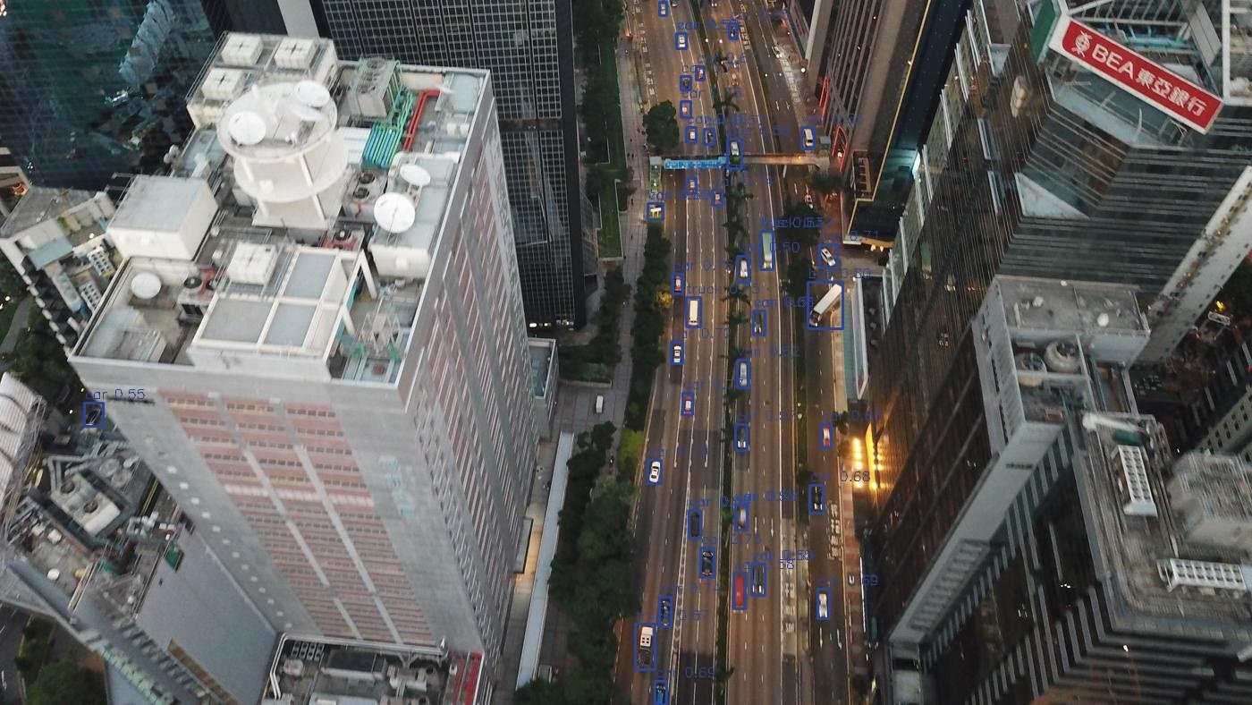
Lastly, let’s see visually the distinction between YOLO11m and D-FINEs. YOLO11m, conf 0.25, nms iou 0.5, latency 13.3ms:

D-FINEs, conf 0.5, no nms, latency 12.3ms:

Each Precision and Recall are larger with the D-FINE mannequin. And it’s additionally sooner. Right here can also be “m” model of D-FINE:

Isn’t it loopy that even that one automobile on the left was detected?
Consideration to information preprocessing
This half can go a bit of bit exterior the scope of the article, however I need to at the least rapidly point out it, as some components will be automated and used within the pipeline. What I positively see as a Laptop Imaginative and prescient engineer is that when engineers don’t spend time working with the information – they don’t get good fashions. You possibly can have all SoTA fashions and all the things finished proper, however rubbish in – rubbish out. So, I all the time pay a ton of consideration to find out how to method the duty and find out how to collect, filter, validate, and annotate the information. Don’t assume that the annotation staff will do all the things proper. Get your fingers soiled and verify manually some portion of the dataset to ensure that annotations are good and picked up photos are consultant.
A number of fast concepts to look into:
- Take away duplicates and close to duplicates from val/take a look at units. The mannequin shouldn’t be validated on one pattern two occasions, and positively, you don’t need to have a knowledge leak, by getting two similar photos, one in coaching and one in validation units.
- Test how small your objects will be. Every little thing not seen to your eye shouldn’t be annotated. Additionally, keep in mind that augmentations will make objects seem even smaller (for instance, mosaic or zoom out). Configure these augmentations accordingly so that you gained’t find yourself with unusably small objects on the picture.
- When you have already got a mannequin for a sure activity and want extra information – strive utilizing your mannequin to pre-annotate new photos. Test instances the place the mannequin fails and collect extra related instances.
The place to begin
I labored quite a bit on this pipeline, and I’m able to share it with everybody who needs to strive it out. It makes use of the SoTA D-FINE mannequin underneath the hood and provides some options that had been absent within the authentic repo (mosaic augmentations, batch accumulation, scheduler, extra metrics, visualization of preprocessed photos and eval predictions, exporting and inference code, higher logging, unified and simplified configuration file).
Right here is the hyperlink to my repo. Right here is the authentic D-FINE repo, the place I additionally contribute. When you want any assist, please contact me on LinkedIn. Thanks to your time!
Citations and acknowledgments
@article{zhu2021detection,
  title={Detection and monitoring meet drones problem},
  creator={Zhu, Pengfei and Wen, Longyin and Du, Dawei and Bian, Xiao and Fan, Heng and Hu, Qinghua and Ling, Haibin},
  journal={IEEE Transactions on Sample Evaluation and Machine Intelligence},
  quantity={44},
  quantity={11},
  pages={7380--7399},
  yr={2021},
  writer={IEEE}
}@misc{peng2024dfine,
title={D-FINE: Redefine Regression Activity in DETRs as Nice-grained Distribution Refinement},
creator={Yansong Peng and Hebei Li and Peixi Wu and Yueyi Zhang and Xiaoyan Solar and Feng Wu},
yr={2024},
eprint={2410.13842},
archivePrefix={arXiv},
primaryClass={cs.CV}
}


