


In July 1959, Arthur Samuel developed one of many first brokers to play the sport of checkers. What constitutes an agent that performs checkers will be greatest described in Samuel’s personal phrases, “…a pc [that] will be programmed so that it’s going to study to play a greater recreation of checkers than will be performed by the one that wrote this system” [1]. The checkers’ agent tries to observe the thought of simulating each doable transfer given the present scenario and deciding on probably the most advantageous one i.e. one which brings the participant nearer to profitable. The transfer’s “advantageousness” is decided by an analysis operate, which the agent improves by way of expertise. Naturally, the idea of an agent just isn’t restricted to the sport of checkers, and plenty of practitioners have sought to match or surpass human efficiency in common video games. Notable examples embrace IBM’s Deep Blue (which managed to defeat Garry Kasparov, a chess world champion on the time), and Tesauro’s TD-Gammon, a temporal-difference method, the place the analysis operate was modelled utilizing a neural community. In truth, TD-Gammon’s taking part in type was so unusual that some specialists even adopted some methods it conjured up [2].
Unsurprisingly, analysis into creating such ‘brokers’ solely skyrocketed, with novel approaches in a position to attain peak human efficiency in complicated video games. On this publish, we discover one such method: the DQN method launched in 2013 by Mnih et al, wherein taking part in Atari video games is approached by way of a synthesis of Deep Neural Networks and TD-Studying (NB: the unique paper got here out in 2013, however we are going to concentrate on the 2015 model which comes with some technical enhancements) [3, 4]. Earlier than we proceed, you must observe that within the ever-expanding house of recent approaches, DQN has been outmoded by quicker and extra refined state-of-the-art strategies. But, it stays a great stepping stone within the subject of Deep Reinforcement Studying, well known for combining deep studying with reinforcement studying. Therefore, readers aiming to dive into Deep-RL are inspired to start with DQN.
This publish is sectioned as follows: first, I outline the issue with taking part in Atari video games and clarify why some conventional strategies will be intractable. Lastly, I current the specifics of the DQN method and dive into the technical implementation.
The Downside At Hand
For the rest of the publish, I’ll assume that the fundamentals of supervised studying, neural networks (primary FFNs and CNNs) and in addition primary reinforcement studying ideas (Bellman equations, TD-learning, Q-learning and many others) If a few of these RL ideas are international to you, then this playlist is an efficient introduction.

Atari is a nostalgia-laden time period, that includes iconic video games akin to Pong, Breakout, Asteroids and plenty of extra. On this publish, we prohibit ourselves to Pong. Pong is a 2-player recreation, the place every participant controls a paddle and may use mentioned paddle to hit the incoming ball. Factors are scored when the opponent is unable to return the ball, in different phrases, the ball goes previous them. A participant wins after they attain 21 factors.
Contemplating the sequential nature of the sport, it may be acceptable to border the issue as an RL drawback, after which apply one of many answer strategies. We will body the sport as an MDP:

The states would signify the present recreation state (the place the ball or participant paddle is and many others, analogous to the thought of a search state). The rewards encapsulate our concept of profitable and the actions correspond to the buttons on the Atari 2600 console. Our aim now turns into discovering a coverage

also called the optimum coverage. Let’s see what may occur if we attempt to practice an agent utilizing some classical RL algorithms.
An easy answer may entail fixing the issue utilizing a tabular method. We may enumerate all states (and actions) and affiliate every state with a corresponding state or state-action worth. We may then apply one of many classical RL strategies (Monte-Carlo, TD-Studying, Worth Iteration and many others), taking a dynamic Programming method. Nevertheless, using this method faces giant pitfalls relatively shortly. What will we take into account as states? What number of states do we’ve to enumerate?
It shortly turns into fairly troublesome to reply these questions. Defining a state turns into troublesome as many components are in play when contemplating the thought of a state (i.e. the states have to be Markovian, encapsulate a search state and many others). What about visible output (frames) to signify a state? In spite of everything that is how we as people work together with Atari video games. We see frames, deduce data concerning the sport state after which select the suitable motion. Nevertheless, there are impossibly many states when utilizing this illustration, which might make our tabular method fairly intractable, memory-wise.
Now for the sake of argument think about that we’ve sufficient reminiscence to carry a desk of this measurement. Even then we would want to discover all of the states a great variety of occasions to get good approximations of the worth operate. We would want to discover all doable states (or state-action) sufficient occasions to reach at a helpful worth. Herein lies the runtime hurdle; it will be fairly infeasible for the values to converge for all of the states within the desk in an affordable period of time as we’ve infinite states.
Maybe as an alternative of framing it as a reinforcement studying drawback, can we as an alternative rephrase it right into a supervised studying drawback? Maybe a formulation wherein the states are samples and the labels are the actions carried out. Even this angle brings forth new issues. Atari video games are inherently sequential, every state is sampled primarily based on the earlier. This breaks the i.i.d assumptions utilized in supervised studying, negatively affecting supervised learning-based options. Equally, we would want to create a hand-labelled dataset, maybe using a human skilled handy label actions for every body. This might be costly and laborious, and nonetheless may yield inadequate outcomes.
Solely counting on both supervised studying or RL could result in inefficient studying, whether or not as a consequence of computational constraints or suboptimal insurance policies. This requires a extra environment friendly method to fixing Atari video games.
DQN: Instinct & Implementation
I assume you’ve got some primary information of PyTorch, Numpy and Python, although I’ll attempt to be as articulate as doable. For these unfamiliar, I like to recommend consulting: pytorch & numpy.
Deep-Q Networks purpose to beat the aforementioned obstacles by way of quite a lot of strategies. Let’s undergo every of the issues step-by-step and tackle how DQN mitigates or solves these challenges.
It’s fairly arduous to provide you with a proper state definition for Atari video games as a consequence of their variety. DQN is designed to work for many Atari video games, and because of this, we want a said formalization that’s suitable with mentioned video games. To this finish, the visible illustration (pixel values) of the video games at any given second are used to style a state. Naturally, this entails a steady state house. This connects to our earlier dialogue on potential methods to signify states.
The problem of steady states is solved by way of operate approximation. Perform approximation (FA) goals to approximate the state-action worth operate instantly utilizing a operate approximation. Let’s undergo the steps to know what the FA does.
Think about that we’ve a community that given a state outputs the worth of being in mentioned state and performing a sure motion. We then choose actions primarily based on the best reward. Nevertheless, this community could be short-sighted, solely bearing in mind one timestep. Can we incorporate doable rewards from additional down the road? Sure we are able to! That is the thought of the anticipated return. From this view, the FA turns into fairly easy to know; we purpose to discover a operate:

In different phrases, a operate which outputs the anticipated return of being in a given state after performing an motion.
This concept of approximation turns into essential as a result of steady nature of the state house. Through the use of a FA, we are able to exploit the thought of generalization. States shut to one another (comparable pixel values) may have comparable Q-values, which means that we don’t must cowl the complete (infinite) state house, tremendously decreasing our computational overhead.
DQN employs FA in tandem with Q-learning. As a small refresher, Q-learning goals to search out the anticipated return for being in a state and performing a sure motion utilizing bootstrapping. Bootstrapping fashions the anticipated return that we talked about utilizing the present Q-function. This ensures that we don’t want to attend until the tip of an episode to replace our Q-function. Q-learning can be 0ff-policy, which implies that the information we use to study the Q-function is totally different from the precise coverage being realized. The ensuing Q-function then corresponds to the optimum Q-function and can be utilized to search out the optimum coverage (simply discover the motion that maximizes the Q-value in a given state). Furthermore, Q-learning is a model-free answer, which means that we don’t must know the dynamics of the atmosphere (transition features and many others) to study an optimum coverage, in contrast to in worth iteration. Thus, DQN can be off-policy and model-free.
Through the use of a neural community as our approximator, we want not assemble a full desk containing all of the states and their respective Q-values. Our neural community will output the Q-value for being a given state and performing a sure motion. From this level on, we confer with the approximator because the Q-network.
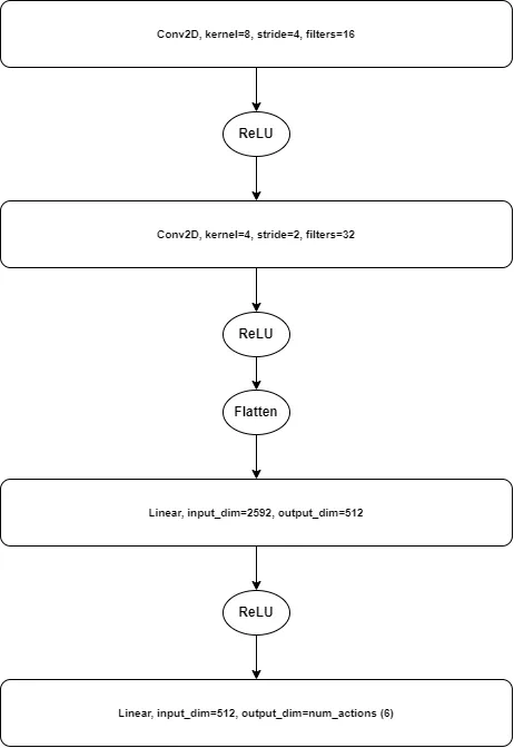
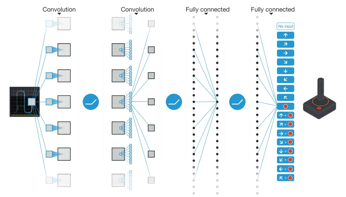
Since our states are outlined by photos, utilizing a primary feed-forward community (FFN) would incur a big computational overhead. For this particular motive, we make use of the usage of a convolutional community, which is significantly better in a position to study the distinct options of every state. The CNNs are in a position to distill the pictures right down to a illustration (that is the thought of illustration studying), which is then fed to a FFN. The neural community structure will be seen above. As an alternative of returning one worth for:

we return an array with every worth similar to a doable motion within the given state (for Pong we are able to carry out 6 actions, so we return 6 values).

Recall that to coach a neural community we have to outline a loss operate that captures our objectives. DQN makes use of the MSE loss operate. For the expected values we the output of our Q-network. For the true values, we use the bootstrapped values. Therefore, our loss operate turns into the next:

If we differentiate the loss operate with respect to the weights we arrive on the following equation.

Plugging this into the stochastic gradient descent (SGD) equation, we arrive at Q-learning [4].
By performing SGD updates utilizing the MSE loss operate, we carry out Q-learning. Nevertheless, that is an approximation of Q-learning, as we don’t replace on a single transfer however as an alternative on a batch of strikes. The expectation is simplified for expedience, although the message stays the identical.
From one other perspective, you can even consider the MSE loss operate as nudging the expected Q-values as near the bootstrapped Q-values (in spite of everything that is what the MSE loss intends). This inadvertently mimics Q-learning, and slowly converges to the optimum Q-function.
By using a operate approximator, we turn into topic to the circumstances of supervised studying, specifically that the information is i.i.d. However within the case of Atari video games (or MDPs) this situation is usually not upheld. Samples from the atmosphere are sequential in nature, making them depending on one another. Equally, because the agent improves the worth operate and updates its coverage, the distribution from which we pattern additionally adjustments, violating the situation of sampling from an an identical distribution.
To resolve this the authors of DQN capitalize on the thought of an expertise replay. This idea is core to maintain the coaching of DQN secure and convergent. An expertise replay is a buffer which shops the tuple (s, a, r, s’, d) the place s, a, r, s’ are returned after performing an motion in an MDP, and d is a boolean representing whether or not the episode has completed or not. The replay has a most capability which is outlined beforehand. It may be easier to think about the replay as a queue or a FIFO knowledge construction; outdated samples are eliminated to make room for brand new samples. The expertise replay is used to pattern a random batch of tuples that are then used for coaching.
The expertise replay helps with the alleviation of two main challenges when utilizing neural community operate approximators with RL issues. The primary offers with the independence of the samples. By randomly sampling a batch of strikes after which utilizing these for coaching we decouple the coaching course of from the sequential nature of Atari video games. Every batch could have actions from totally different timesteps (and even totally different episodes), giving a stronger semblance of independence.
Secondly, the expertise replay addresses the problem of non-stationarity. Because the agent learns, adjustments in its behaviour are mirrored within the knowledge. That is the thought of non-stationarity; the distribution of knowledge adjustments over time. By reusing samples within the replay and utilizing a FIFO construction, we restrict the hostile results of non-stationarity on coaching. The distribution of the information nonetheless adjustments, however slowly and its results are much less impactful. Since Q-learning is an off-policy algorithm, we nonetheless find yourself studying the optimum coverage, making this a viable answer. These adjustments enable for a extra secure coaching process.
As a serendipitous aspect impact, the expertise replay additionally permits for higher knowledge effectivity. Earlier than coaching examples had been discarded after getting used for a single replace step. Nevertheless, by way of the usage of an expertise replay, we are able to reuse strikes that we’ve made previously for updates.
A change made within the 2015 Nature model of DQN was the introduction of a goal community. Neural networks are fickle; slight adjustments within the weights can introduce drastic adjustments within the output. That is unfavourable for us, as we use the outputs of the Q-network to bootstrap our targets. If the targets are vulnerable to giant adjustments, it should destabilize coaching, which naturally we need to keep away from. To alleviate this difficulty, the authors introduce a goal community, which copies the weights of the Q-network each set quantity of timesteps. Through the use of the goal community for bootstrapping, our bootstrapped targets are much less unstable, making coaching extra environment friendly.
Lastly, the DQN authors stack 4 consecutive frames after executing an motion. This comment is made to make sure the Markovian property holds [9]. A singular body omits many particulars of the sport state akin to the speed and course of the ball. A stacked illustration is ready to overcome these obstacles, offering a holistic view of the sport at any given timestep.
With this, we’ve lined many of the main strategies used for coaching a DQN agent. Let’s go over the coaching process. The process will likely be extra of an outline, and we’ll iron out the main points within the implementation part.
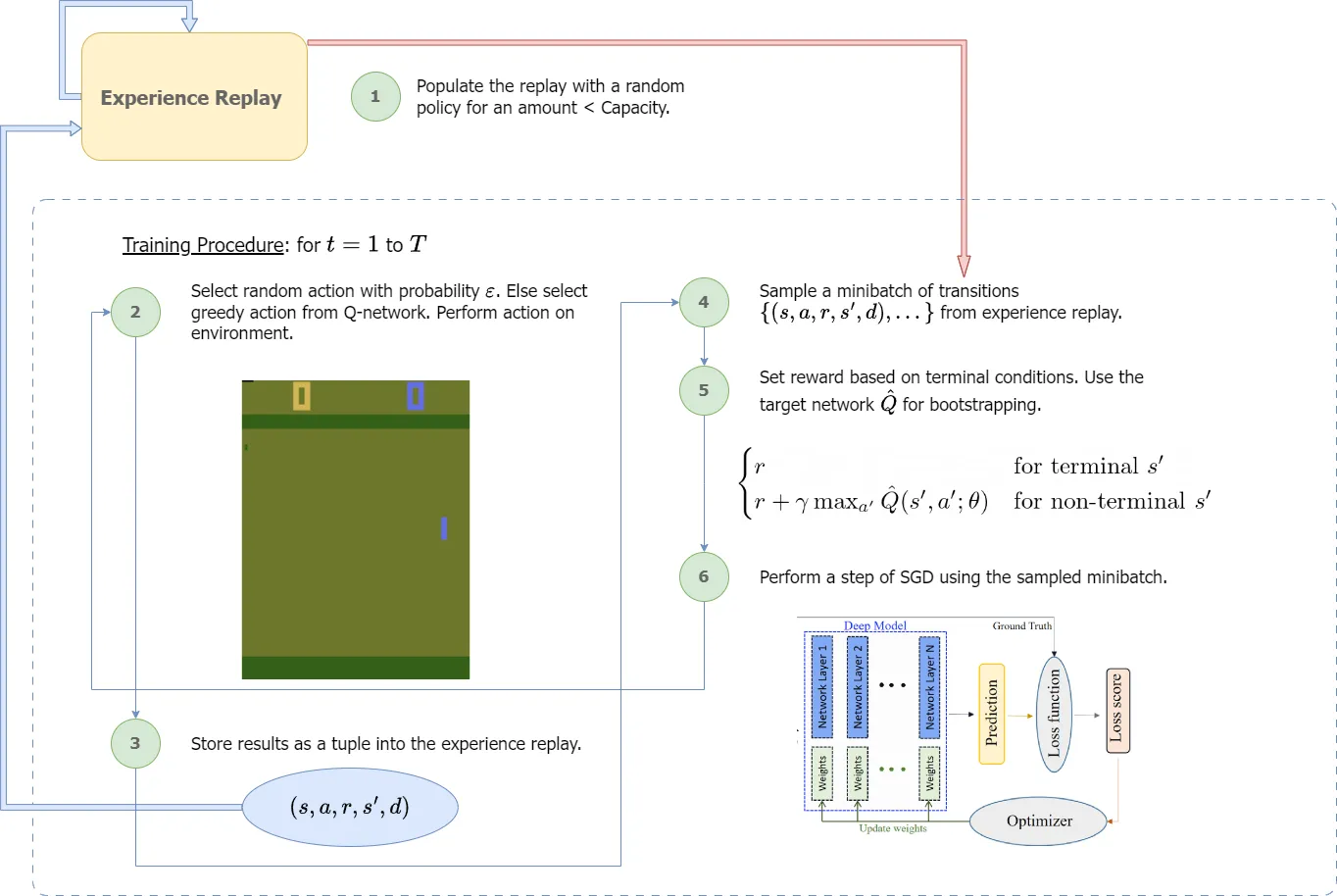
One essential clarification arises from step 2. On this step, we carry out a course of known as ε-greedy motion choice. In ε-greedy, we randomly select an motion with likelihood ε, and in any other case select the absolute best motion (in line with our realized Q-network). Selecting an acceptable ε permits for the adequate exploration of actions which is essential to converge to a dependable Q-function. We frequently begin with a excessive ε and slowly decay this worth over time.
Implementation
If you wish to observe together with my implementation of DQN then you will have the next libraries (other than Numpy and PyTorch). I present a concise rationalization of their use.
- Arcade Studying Surroundings → ALE is a framework that permits us to work together with Atari 2600 environments. Technically we interface ALE by way of gymnasium, an API for RL environments and benchmarking.
- StableBaselines3 → SB3 is a deep reinforcement studying framework with a backend designed in Pytorch. We’ll solely want this for some preprocessing wrappers.
Let’s import all the crucial libraries.
import numpy as np
import time
import torch
import torch.nn as nn
import gymnasium as gymnasium
import ale_py

from collections import deque # FIFO queue knowledge structurefrom tqdm import tqdm  # progress barsfrom gymnasium.wrappers import FrameStack
from gymnasium.wrappers.frame_stack import LazyFrames
from stable_baselines3.frequent.atari_wrappers import (
  AtariWrapper,
  FireResetEnv,
)

gymnasium.register_envs(ale_py) # we have to register ALE with gymnasium

# use cuda you probably have it in any other case cpu
machine="cuda" if torch.cuda.is_available() else 'cpu'
machine
First, we assemble an atmosphere, utilizing the ALE framework. Since we’re working with pong we create an atmosphere with the title PongNoFrameskip-v4. With this, we are able to create an atmosphere utilizing the next code:
env = gymnasium.make('PongNoFrameskip-v4', render_mode="rgb_array")The rgb_array parameter tells ALE to return pixel values as an alternative of RAM codes (which is the default). The code to work together with the Atari turns into very simple with gymnasium. The next excerpt encapsulates many of the utilities that we’ll want from gymnasium.
# this code restarts/begins a atmosphere to the start of an episode
commentary, _ = env.reset()
for _ in vary(100):  # variety of timesteps
  # randomly get an motion from doable actions
  motion = env.action_space.pattern()
  # take a step utilizing the given motion
  # observation_prime refers to s', terminated and truncated confer with
  # whether or not an episode has completed or been reduce quick
  observation_prime, reward, terminated, truncated, _ = env.step(motion)
  commentary = observation_prime
With this, we’re given states (we title them observations) with the form (210, 160, 3). Therefore the states are RGB photos with the form 210×160. An instance will be seen in Determine 2. When coaching our DQN agent, a picture of this measurement provides pointless computational overhead. The same commentary will be made about the truth that the frames are RGB (3 channels).
To resolve this, we downsample the body right down to 84×84 and rework it into grayscale. We will do that by using a wrapper from SB3, which does this for us. Now each time we carry out an motion our output will likely be in grayscale (with 1 channel) and of measurement 84×84.
env = AtariWrapper(env, terminal_on_life_loss=False, frame_skip=4)The wrapper above does greater than downsample and switch our body into grayscale. Let’s go over another adjustments the wrapper introduces.
- Noop Reset → The beginning state of every Atari recreation is deterministic, i.e. you begin on the similar state every time the sport ends. With this the agent could study to memorize a sequence of actions from the beginning state, leading to a sub-optimal coverage. To stop this, we carry out no actions for a set quantity of timesteps to start with.
- Body Skipping → Within the ALE atmosphere every body wants an motion. As an alternative of selecting an motion at every body, we choose an motion and repeat it for a set variety of timesteps. That is the thought of body skipping and permits for smoother transitions.
- Max-pooling → As a result of method wherein ALE/Atari renders its frames and the downsampling, it’s doable that we encounter flickering. To resolve this we take the max over two consecutive frames.
- Terminal Life on Loss → Many Atari video games don’t finish when the participant dies. Contemplate Pong, no participant wins till the rating hits 21. Nevertheless, by default brokers may take into account the lack of life as the tip of an episode, which is undesirable. This wrapper counteracts this and ends the episode when the sport is actually over.
- Clip Reward → The gradients are extremely delicate to the magnitude of the rewards. To keep away from unstable updates, we clip the rewards to be between {-1, 0, 1}.
Other than these we additionally introduce a further body stack wrapper (FrameStack). This performs what was mentioned above, stacking 4 frames on high of every to maintain the states Markovian. The ALE atmosphere returns LazyFrames, that are designed to be extra reminiscence environment friendly, as the identical body may happen a number of occasions. Nevertheless, they don’t seem to be suitable with most of the operations that we carry out all through the coaching process. To transform LazyFrames into usable objects, we apply a customized wrapper which converts an commentary to Numpy earlier than returning it to us. The code is proven beneath.
class LazyFramesToNumpyWrapper(gymnasium.ObservationWrapper): # subclass obswrapper
  def __init__(self, env):
      tremendous().__init__(env)
      self.env = env # the atmosphere that we need to convert

  def commentary(self, commentary):
      # if its a LazyFrames object then flip it right into a numpy array
      if isinstance(commentary, LazyFrames):
          return np.array(commentary)
      return commentary
Let’s mix all the wrappers into one operate that returns an atmosphere that does all the above.
def make_env(recreation, render="rgb_array"):
  env = gymnasium.make(recreation, render_mode=render)
  env = AtariWrapper(env, terminal_on_life_loss=False, frame_skip=4)
  env = FrameStack(env, num_stack=4)
  env = LazyFramesToNumpyWrapper(env)
  # generally a atmosphere wants that the fireplace button be
  # pressed to start out the sport, this makes certain that recreation is began when wanted
  if "FIRE" in env.unwrapped.get_action_meanings():
      env = FireResetEnv(env)
  return env
These adjustments are derived from the 2015 Nature paper and assist to stabilize coaching [3]. The interfacing with gymnasium stays the identical as proven above. An instance of the preprocessed states will be seen in Determine 7.
Now that we’ve an acceptable atmosphere let’s transfer on to create the replay buffer.
class ReplayBuffer:

  def __init__(self, capability, machine):
      self.capability = capability
      self._buffer =  np.zeros((capability,), dtype=object) # shops the tuples
      self._position = 0 # hold observe of the place we're
      self._size = 0
      self.machine = machine

  def retailer(self, expertise):
      """Provides a brand new expertise to the buffer,
        overwriting outdated entries when full."""
      idx = self._position % self.capability # get the index to switch
      self._buffer[idx] = expertise
      self._position += 1
      self._size = min(self._size + 1, self.capability) # max measurement is the capability

  def pattern(self, batch_size):
      """ Pattern a batch of tuples and cargo it onto the machine
      """
      # if the buffer just isn't full capability then return all the pieces we've
      buffer = self._buffer[0:min(self._position-1, self.capacity-1)]
      # minibatch of tuples
      batch = np.random.alternative(buffer, measurement=[batch_size], exchange=True)

      # we have to return the objects as torch tensors, therefore we delegate
      # this process to the rework operate
      return (
          self.rework(batch, 0, form=(batch_size, 4, 84, 84), dtype=torch.float32),
          self.rework(batch, 1, form=(batch_size, 1), dtype=torch.int64),
          self.rework(batch, 2, form=(batch_size, 1), dtype=torch.float32),
          self.rework(batch, 3, form=(batch_size, 4, 84, 84), dtype=torch.float32),
          self.rework(batch, 4, form=(batch_size, 1), dtype=torch.bool)
      )

  def rework(self, batch, index, form, dtype):
      """ Rework a handed batch right into a torch tensor for a given axis.
      E.g. if index 0 of a tuple means the state then we return all states
      as a torch tensor. We additionally return a specified form.
      """
      # reshape the tensors as wanted
      batched_values = np.array([val[index] for val in batch]).reshape(form)
      # convert to torch tensors
      batched_values = torch.as_tensor(batched_values, dtype=dtype, machine=self.machine)
      return batched_values

  # beneath are some magic strategies I used for debugging, not essential
  # they simply flip the article into an arraylike object
  def __len__(self):
      return self._size

  def __getitem__(self, index):
      return self._buffer[index]

  def __setitem__(self, index, worth: tuple):
      self._buffer[index] = worth
The replay buffer works by allocating house within the reminiscence for the given capability. We keep a pointer that retains observe of the variety of objects added. Each time a brand new tuple is added we exchange the oldest tuples with the brand new ones. To pattern a minibatch, we first randomly pattern a minibatch in numpy after which convert it into torch tensors, additionally loading it to the suitable machine.
Among the features of the replay buffer are impressed by [8]. The replay buffer proved to be the most important bottleneck in coaching the agent, and thus small speed-ups within the code proved to be monumentally essential. An alternate technique which makes use of an deque object to carry the tuples will also be used. If you’re creating your personal buffer, I’d emphasize that you simply spend slightly extra time to make sure its effectivity.
We will now use this to create a operate that creates a buffer and preloads a given variety of tuples with a random coverage.
def load_buffer(preload, capability, recreation, *, machine):
  # make the atmosphere
  env = make_env(recreation)
  # create the buffer
  buffer = ReplayBuffer(capability,machine=machine)

  # begin the atmosphere
  commentary, _ = env.reset()
  # run for so long as the required preload
  for _ in tqdm(vary(preload)):
      # pattern random motion -> random coverage
      motion = env.action_space.pattern()

      observation_prime, reward, terminated, truncated, _ = env.step(motion)

      # retailer the outcomes from the motion as a python tuple object
      buffer.retailer((
          commentary.squeeze(), # squeeze will take away the pointless grayscale channel
          motion,
          reward,
          observation_prime.squeeze(),
          terminated or truncated))
      # set outdated commentary to be new observation_prime
      commentary = observation_prime

      # if the episode is completed, then restart the atmosphere
      carried out = terminated or truncated
      if carried out:
          commentary, _ = env.reset()

  # return the env AND the loaded buffer
  return buffer, env
The operate is kind of easy, we create a buffer and atmosphere object after which preload the buffer utilizing a random coverage. Notice that we squeeze the observations to take away the redundant coloration channel. Let’s transfer on to the subsequent step and outline the operate approximator.
class DQN(nn.Module):

  def __init__(
      self,
      env,
      in_channels = 4, # variety of stacked frames
      hidden_filters = [16, 32],
      start_epsilon = 0.99, # beginning epsilon for epsilon-decay
      max_decay = 0.1, # finish epsilon-decay
      decay_steps = 1000, # how lengthy to achieve max_decay
      *args,
      **kwargs
  ) -> None:
      tremendous().__init__(*args, **kwargs)

      # instantiate occasion vars
      self.start_epsilon = start_epsilon
      self.epsilon = start_epsilon
      self.max_decay = max_decay
      self.decay_steps = decay_steps
      self.env = env
      self.num_actions = env.action_space.n

      # Sequential is an arraylike object that permits us to
      # carry out the ahead move in a single line
      self.layers = nn.Sequential(
          nn.Conv2d(in_channels, hidden_filters[0], kernel_size=8, stride=4),
          nn.ReLU(),
          nn.Conv2d(hidden_filters[0], hidden_filters[1], kernel_size=4, stride=2),
          nn.ReLU(),
          nn.Flatten(start_dim=1),
          nn.Linear(hidden_filters[1] * 9 * 9, 512), # the ultimate worth is calculated by utilizing the equation for CNNs
          nn.ReLU(),
          nn.Linear(512, self.num_actions)
      )

      # initialize weights utilizing he initialization
      # (pytorch already does this for conv layers however not linear layers)
      # this isn't crucial and nothing you should fear about
      self.apply(self._init)

  def ahead(self, x):
      """ Ahead move. """
      # the /255.0 performs normalization of pixel values to be in [0.0, 1.0]
      return self.layers(x / 255.0)

  def epsilon_greedy(self, state, dim=1):
      """Epsilon grasping. Randomly choose worth with prob e,
        else select grasping motion"""

      rng = np.random.random() # get random worth between [0, 1]

      if rng < self.epsilon: # for prob below e
          # random pattern and return as torch tensor
          motion = self.env.action_space.pattern()
          motion = torch.tensor(motion)
      else:
          # use torch no grad to verify no gradients are amassed for this
          # ahead move
          with torch.no_grad():
              q_values = self(state)
          # select greatest motion
          motion = torch.argmax(q_values, dim=dim)

      return motion

  def epsilon_decay(self, step):
      # linearly lower epsilon
      self.epsilon = self.max_decay + (self.start_epsilon - self.max_decay) * max(0, (self.decay_steps - step) / self.decay_steps)

  def _init(self, m):
    # initialize layers utilizing he init
    if isinstance(m, (nn.Linear, nn.Conv2d)):
      nn.init.kaiming_normal_(m.weight, nonlinearity='relu')
      if m.bias just isn't None:
        nn.init.zeros_(m.bias)
That covers the mannequin structure. I used a linear ε-decay scheme, however be at liberty to strive one other. We will additionally create an auxiliary class that retains observe of essential metrics. The category retains observe of rewards obtained for the previous couple of episodes together with the respective lengths of mentioned episodes.
class MetricTracker:
  def __init__(self, window_size=100):
      # the scale of the historical past we use to trace stats
      self.window_size = window_size
      self.rewards = deque(maxlen=window_size)
      self.current_episode_reward = 0

  def add_step_reward(self, reward):
      # add obtained reward to the present reward
      self.current_episode_reward += reward

  def end_episode(self):
      # add reward for episode to historical past
      self.rewards.append(self.current_episode_reward)
      # reset metrics
      self.current_episode_reward = 0

  # property simply makes it in order that we are able to return this worth with out
  # having to name it as a operate
  @property
  def avg_reward(self):
      return np.imply(self.rewards) if self.rewards else 0
Nice! Now we’ve all the pieces we have to begin coaching our agent. Let’s outline the coaching operate and go over the way it works. Earlier than that, we have to create the mandatory objects to move into our coaching operate together with some hyperparameters. A small observe: within the paper the authors use RMSProp, however as an alternative we’ll use Adam. Adam proved to work for me with the given parameters, however you might be welcome to strive RMSProp or different variations.
TIMESTEPS = 6000000 # whole variety of timesteps for coaching
LR = 2.5e-4 # studying charge
BATCH_SIZE = 64 # batch measurement, change primarily based in your {hardware}
C = 10000 # the interval at which we replace the goal community
GAMMA = 0.99 # the low cost worth
TRAIN_FREQ = 4 # within the paper the SGD updates are made each 4 actions
DECAY_START = 0 # when to start out e-decay
FINAL_ANNEAL = 1000000 # when to cease e-decay

# load the buffer
buffer_pong, env_pong = load_buffer(50000, 150000, recreation="PongNoFrameskip-v4")

# create the networks, push the weights of the q_network onto the goal community
q_network_pong = DQN(env_pong, decay_steps=FINAL_ANNEAL).to(machine)
target_network_pong = DQN(env_pong, decay_steps=FINAL_ANNEAL).to(machine)
target_network_pong.load_state_dict(q_network_pong.state_dict())

# create the optimizer
optimizer_pong = torch.optim.Adam(q_network_pong.parameters(), lr=LR)

# metrics class instantiation
metrics = MetricTracker()
def practice(
env,
title, # title of the agent, used to save lots of the agent
q_network,
target_network,
optimizer,
timesteps,
replay, # handed buffer
metrics, # metrics class
train_freq, # this parameter works complementary to border skipping
batch_size,
gamma, # low cost parameter
decay_start,
C,
save_step=850000, # I like to recommend setting this one excessive or else a number of fashions will likely be saved
):
loss_func = nn.MSELoss() # create the loss object
start_time = time.time() # to verify velocity of the coaching process
episode_count = 0
best_avg_reward = -float('inf')
# reset the env
obs, _ = env.reset()
for step in vary(1, timesteps+1): # begin from 1 only for printing progress
# we have to move tensors of measurement (batch_size, ...) to torch
# however the commentary is only one so it does not have that dim
# so we add it artificially (step 2 in process)
batched_obs = np.expand_dims(obs.squeeze(), axis=0)
# carry out e-greedy on the commentary and convert the tensor into numpy and ship it to the cpu
motion = q_network.epsilon_greedy(torch.as_tensor(batched_obs, dtype=torch.float32, machine=machine)).cpu().merchandise()
# take an motion
obs_prime, reward, terminated, truncated, _ = env.step(motion)
# retailer the tuple (step 3 within the process)
replay.retailer((obs.squeeze(), motion, reward, obs_prime.squeeze(), terminated or truncated))
metrics.add_step_reward(reward)
obs = obs_prime
# practice each 4 steps as per the paper
if step % train_freq == 0:
# pattern tuples from the replay (step 4 within the process)
observations, actions, rewards, observation_primes, dones = replay.pattern(batch_size)
# we do not need to accumulate gradients for this operation so use no_grad
with torch.no_grad():
q_values_minus = target_network(observation_primes)
# get the max over the goal community
boostrapped_values = torch.amax(q_values_minus, dim=1, keepdim=True)
# this line principally makes in order that for each pattern within the minibatch which signifies
# that the episode is completed, we return the reward, else we return the
# the bootstrapped reward (step 5 within the process)
y_trues = torch.the place(dones, rewards, rewards + gamma * boostrapped_values)
y_preds = q_network(observations)
# compute the loss
# the collect will get the values of the q_network similar to the
# motion taken
loss = loss_func(y_preds.collect(1, actions), y_trues)
# set the grads to 0, and carry out the backward move (step 6 within the process)
optimizer.zero_grad()
loss.backward()
optimizer.step()
# begin the e-decay
if step > decay_start:
q_network.epsilon_decay(step)
target_network.epsilon_decay(step)
# if the episode is completed then we print some metrics
if terminated or truncated:
# compute steps per sec
elapsed_time = time.time() - start_time
steps_per_sec = step / elapsed_time
metrics.end_episode()
episode_count += 1
# reset the atmosphere
obs, _ = env.reset()
# save a mannequin if above save_step and if the common reward has improved
# that is type of like early-stopping, however we do not cease we simply save a mannequin
if metrics.avg_reward > best_avg_reward and step > save_step:
best_avg_reward = metrics.avg_reward
torch.save({
'step': step,
'model_state_dict': q_network.state_dict(),
'optimizer_state_dict': optimizer.state_dict(),
'avg_reward': metrics.avg_reward,
}, f"fashions/{title}_dqn_best_{step}.pth")
# print some metrics
print(f"rStep: {step:,}/{timesteps:,} | "
f"Episodes: {episode_count} | "
f"Avg Reward: {metrics.avg_reward:.1f} | "
f"Epsilon: {q_network.epsilon:.3f} | "
f"Steps/sec: {steps_per_sec:.1f}", finish="r")
# replace the goal community
if step % C == 0:
target_network.load_state_dict(q_network.state_dict())The coaching process carefully follows Determine 6 and the algorithm described within the paper [4]. We first create the mandatory objects such because the loss operate and many others and reset the atmosphere. Then we are able to begin the coaching loop, by utilizing the Q-network to offer us an motion primarily based on the ε-greedy coverage. We simulate the atmosphere one step ahead utilizing the motion and push the resultant tuple onto the replay. If the replace frequency situation is met, we are able to proceed with a coaching step. The motivation behind the replace frequency component is one thing I’m not 100% assured in. At present, the reason I can present revolves round computational effectivity: coaching each 4 steps as an alternative of each step majorly hastens the algorithm and appears to work comparatively nicely. Within the replace step itself, we pattern a minibatch of tuples and run the mannequin ahead to provide predicted Q-values. We then create the goal values (the bootstrapped true labels) utilizing the piecewise operate in step 5 in Determine 6. Performing an SGD step turns into fairly easy from this level, since we are able to depend on autograd to compute the gradients and the optimizer to replace the parameters.
In case you adopted alongside till now, you should utilize the next check operate to check your saved mannequin.
def check(recreation, mannequin, num_eps=2):
  # render human opens an occasion of the sport so you may see it
  env_test = make_env(recreation, render="human")

  # load the mannequin
  q_network_trained = DQN(env_test)
  q_network_trained.load_state_dict(torch.load(mannequin, weights_only=False)['model_state_dict'])
  q_network_trained.eval() # set the mannequin to inference mode (no gradients and many others)
  q_network_trained.epsilon = 0.05 # a small quantity of stochasticity


  rewards_list = []

  # run for set quantity of episodes
  for episode in vary(num_eps):
      print(f'Episode {episode}', finish='r', flush=True)

      # reset the env
      obs, _ = env_test.reset()
      carried out = False
      total_reward = 0

      # till the episode just isn't carried out, carry out the motion from the q-network
      whereas not carried out:
          batched_obs = np.expand_dims(obs.squeeze(), axis=0)
          motion = q_network_trained.epsilon_greedy(torch.as_tensor(batched_obs, dtype=torch.float32)).cpu().merchandise()

          next_observation, reward, terminated, truncated, _ = env_test.step(motion)
          total_reward += reward
          obs = next_observation

          carried out = terminated or truncated

      rewards_list.append(total_reward)

  # shut the atmosphere, since we use render human
  env_test.shut()
  print(f'Common episode reward achieved: {np.imply(rewards_list)}')
Right here’s how you should utilize it:
# be sure to use your newest mannequin! I additionally renamed my mannequin path so
# take that into consideration
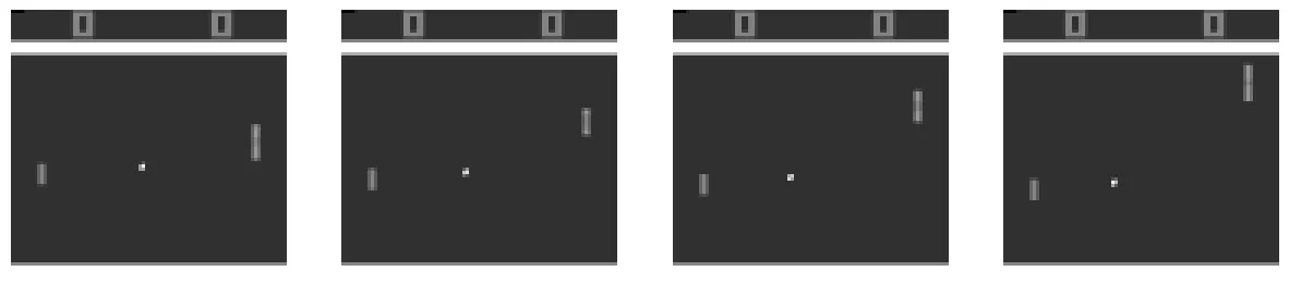
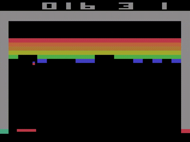
check('PongNoFrameskip-v4', 'fashions/pong_dqn_best_6M.pth')That’s all the pieces for the code! You possibly can see a educated agent beneath in Determine 8. It behaves fairly just like a human may play Pong, and is ready to (persistently) beat the AI on the simplest problem. This naturally invitations the query, how nicely does it carry out on increased difficulties? Attempt it out utilizing your personal agent or my educated one!

A further agent was educated on the sport Breakout as nicely, the agent will be seen in Determine 9. As soon as once more, I used the default mode and problem. It may be attention-grabbing to see how nicely it performs in several modes or difficulties.
Abstract
DQN solves the problem of coaching brokers to play Atari video games. Through the use of a FA, expertise replay and many others, we’re in a position to practice an agent that mimics and even surpasses human efficiency in Atari video games [3]. Deep-RL brokers will be finicky and also you may need observed that we use a lot of strategies to make sure that coaching is secure. If issues are going improper along with your implementation it may not damage to take a look at the main points once more.
If you wish to take a look at the code for my implementation you should utilize this hyperlink. The repo additionally accommodates code to coach your personal mannequin on the sport of your alternative (so long as it’s in ALE), in addition to the educated weights for each Pong and Breakout.
I hope this was a useful introduction to coaching DQN brokers. To take issues to the subsequent degree possibly you may attempt to tweak particulars to beat the upper difficulties. If you wish to look additional, there are numerous extensions to DQN you may discover, akin to Dueling DQNs, Prioritized Replay and many others.
References
[1] A. L. Samuel, “Some Research in Machine Studying Utilizing the Recreation of Checkers,” IBM Journal of Analysis and Improvement, vol. 3, no. 3, pp. 210–229, 1959. doi:10.1147/rd.33.0210.
[2] Sammut, Claude; Webb, Geoffrey I., eds. (2010), “TD-Gammon”, Encyclopedia of Machine Studying, Boston, MA: Springer US, pp. 955–956, doi:10.1007/978–0–387–30164–8_813, ISBN 978–0–387–30164–8, retrieved 2023–12–25
[3] Mnih, Volodymyr, Koray Kavukcuoglu, David Silver, Andrei A. Rusu, Joel Veness, Marc G. Bellemare, … and Demis Hassabis. “Human-Stage Management by way of Deep Reinforcement Studying.” Nature 518, no. 7540 (2015): 529–533. https://doi.org/10.1038/nature14236
[4] Mnih, Volodymyr, Koray Kavukcuoglu, David Silver, Andrei A. Rusu, Joel Veness, Marc G. Bellemare, … and Demis Hassabis. “Enjoying Atari with Deep Reinforcement Studying.” arXiv preprint arXiv:1312.5602 (2013). https://arxiv.org/abs/1312.5602
[5] Sutton, Richard S., and Andrew G. Barto. Reinforcement Studying: An Introduction. 2nd ed., MIT Press, 2018.
[6] Russell, Stuart J., and Peter Norvig. Synthetic Intelligence: A Trendy Method. 4th ed., Pearson, 2020.
[7] Goodfellow, I., Bengio, Y., & Courville, A. (2016). Deep Studying. MIT Press.
[8] Bailey, Jay. Deep Q-Networks Defined. 13 Sept. 2022, www.lesswrong.com/posts/kyvCNgx9oAwJCuevo/deep-q-networks-explained.
[9] Hausknecht, M., & Stone, P. (2015). Deep recurrent Q-learning for partially observable MDPs. arXiv preprint arXiv:1507.06527. https://arxiv.org/abs/1507.06527


