


A workflow and code walkthrough for constructing a Bayesian regression mannequin in STAN
Observe: Try my earlier article for a sensible dialogue on why Bayesian modeling stands out as the proper alternative on your activity.
This tutorial will deal with a workflow + code walkthrough for constructing a Bayesian regression mannequin in STAN, a probabilistic programming language. STAN is broadly adopted and interfaces along with your language of alternative (R, Python, shell, MATLAB, Julia, Stata). See the set up information and documentation.
I’ll use Pystan for this tutorial, just because I code in Python. Even in case you use one other language, the overall Bayesian practices and STAN language syntax I’ll focus on right here doesn’t differ a lot.
For the extra hands-on reader, here’s a hyperlink to the pocket book for this tutorial, a part of my Bayesian modeling workshop at Northwestern College (April, 2024).
Let’s dive in!
Lets discover ways to construct a easy linear regression mannequin, the bread and butter of any statistician, the Bayesian approach. Assuming a dependent variable Y and covariate X, I suggest the next easy model-
Y = α + β * X + ϵ
The place ⍺ is the intercept, β is the slope, and ϵ is a few random error. Assuming that,
ϵ ~ Regular(0, σ)
we are able to present that
Y ~ Regular(α + β * X, σ)
We are going to discover ways to code this mannequin kind in STAN.
Generate Information
First, let’s generate some pretend information.
#Mannequin Parameters
alpha = 4.0  #intercept
beta = 0.5 #slope
sigma = 1.0 #error-scale
#Generate pretend information
x =  8 * np.random.rand(100)
y = alpha + beta * x
y = np.random.regular(y, scale=sigma) #noise
#visualize generated information
plt.scatter(x, y, alpha = 0.8)

Now that we have now some information to mannequin, let’s dive into methods to construction it and go it to STAN together with modeling directions. That is carried out through the mannequin string, which generally comprises 4 (often extra) blocks- information, parameters, mannequin, and generated portions. Let’s focus on every of those blocks intimately.
DATA block
information {                    //enter the info to STAN
int N;
vector[N] x;
vector[N] y;
}
The information block is maybe the only, it tells STAN internally what information it ought to anticipate, and in what format. As an illustration, right here we pass-
N: the dimensions of our dataset as sort int. The
x: the covariate as a vector of size N.
y: the dependent as a vector of size N.
See docs right here for a full vary of supported information sorts. STAN gives assist for a variety of sorts like arrays, vectors, matrices and many others. As we noticed above, STAN additionally has assist for encoding limits on variables. Encoding limits is really useful! It results in higher specified fashions and simplifies the probabilistic sampling processes working beneath the hood.
Mannequin Block
Subsequent is the mannequin block, the place we inform STAN the construction of our mannequin.
//easy mannequin block
mannequin {
//priors
alpha ~ regular(0,10);
beta ~ regular(0,1); //mannequin
y ~ regular(alpha + beta * x, sigma);
}
The mannequin block additionally comprises an necessary, and sometimes complicated, factor: prior specification. Priors are a quintessential a part of Bayesian modeling, and have to be specified suitably for the sampling activity.
See my earlier article for a primer on the position and instinct behind priors. To summarize, the prior is a presupposed purposeful kind for the distribution of parameter values — usually referred to, merely, as prior perception. Regardless that priors don’t have to precisely match the ultimate resolution, they have to permit us to pattern from it.
In our instance, we use Regular priors of imply 0 with completely different variances, relying on how positive we’re of the equipped imply worth: 10 for alpha (very uncertain), 1 for beta (considerably positive). Right here, I equipped the overall perception that whereas alpha can take a variety of various values, the slope is mostly extra contrained and received’t have a big magnitude.
Therefore, within the instance above, the prior for alpha is ‘weaker’ than beta.
As fashions get extra difficult, the sampling resolution area expands, and supplying beliefs beneficial properties significance. In any other case, if there isn’t any sturdy instinct, it’s good apply to only provide much less perception into the mannequin i.e. use a weakly informative prior, and stay versatile to incoming information.
The shape for y, which you might need acknowledged already, is the usual linear regression equation.
Generated Portions
Lastly, we have now our block for generated portions. Right here we inform STAN what portions we wish to calculate and obtain as output.
generated portions {    //get portions of curiosity from fitted mannequin
vector[N] yhat;
vector[N] log_lik;
for (n in 1:N) alpha + x[n] * beta, sigma);
//chance of knowledge given the mannequin and parameters

}
Observe: STAN helps vectors to be handed both straight into equations, or as iterations 1:N for every factor n. In apply, I’ve discovered this assist to vary with completely different variations of STAN, so it’s good to attempt the iterative declaration if the vectorized model fails to compile.
Within the above example-
yhat: generates samples for y from the fitted parameter values.
log_lik: generates chance of knowledge given the mannequin and fitted parameter worth.
The aim of those values will probably be clearer after we speak about mannequin analysis.
Altogether, we have now now totally specified our first easy Bayesian regression mannequin:
mannequin = """
information {                    //enter the info to STAN
int N;
vector[N] x;
vector[N] y;
}
parameters {
actual alpha;
actual beta;
actualsigma; mannequin {
}
alpha ~ regular(0,10);
beta ~ regular(0,1);
y ~ regular(alpha + beta * x, sigma);
}generated portions {
vector[N] yhat;
vector[N] log_lik;for (n in 1:N) alpha + x[n] * beta, sigma);
}
"""
All that continues to be is to compile the mannequin and run the sampling.
#STAN takes information as a dict
information = {'N': len(x), 'x': x, 'y': y}
STAN takes enter information within the type of a dictionary. It will be significant that this dict comprises all of the variables that we instructed STAN to anticipate within the model-data block, in any other case the mannequin received’t compile.
#parameters for STAN becoming
chains = 2
samples = 1000
warmup = 10
# set seed
# Compile the mannequin
posterior = stan.construct(mannequin, information=information, random_seed = 42)
# Prepare the mannequin and generate samples
match = posterior.pattern(num_chains=chains, num_samples=samples)The .pattern() technique parameters management the Hamiltonian Monte Carlo (HMC) sampling course of, the place —
- num_chains: is the variety of instances we repeat the sampling course of.
- num_samples: is the variety of samples to be drawn in every chain.
- warmup: is the variety of preliminary samples that we discard (because it takes a while to achieve the overall neighborhood of the answer area).
Realizing the proper values for these parameters is determined by each the complexity of our mannequin and the assets obtainable.
Larger sampling sizes are in fact very best, but for an ill-specified mannequin they are going to show to be simply waste of time and computation. Anecdotally, I’ve had massive information fashions I’ve needed to wait per week to complete working, solely to seek out that the mannequin didn’t converge. Is is necessary to begin slowly and sanity examine your mannequin earlier than working a full-fledged sampling.
Mannequin Analysis
The generated portions are used for
- evaluating the goodness of match i.e. convergence,
- predictions
- mannequin comparability
Convergence
Step one for evaluating the mannequin, within the Bayesian framework, is visible. We observe the sampling attracts of the Hamiltonian Monte Carlo (HMC) sampling course of.

In simplistic phrases, STAN iteratively attracts samples for our parameter values and evaluates them (HMC does approach extra, however that’s past our present scope). For a great match, the pattern attracts should converge to some widespread normal space which might, ideally, be the worldwide optima.
The determine above reveals the sampling attracts for our mannequin throughout 2 impartial chains (pink and blue).
- On the left, we plot the general distribution of the fitted parameter worth i.e. the posteriors. We anticipate a regular distribution if the mannequin, and its parameters, are properly specified. (Why is that? Nicely, a standard distribution simply implies that there exist a sure vary of greatest match values for the parameter, which speaks in assist of our chosen mannequin kind). Moreover, we must always anticipate a substantial overlap throughout chains IF the mannequin is converging to an optima.
- On the proper, we plot the precise samples drawn in every iteration (simply to be additional positive). Right here, once more, we want to see not solely a slender vary but additionally quite a lot of overlap between the attracts.
Not all analysis metrics are visible. Gelman et al. [1] additionally suggest the Rhat diagnostic which important is a mathematical measure of the pattern similarity throughout chains. Utilizing Rhat, one can outline a cutoff level past which the 2 chains are judged too dissimilar to be converging. The cutoff, nonetheless, is difficult to outline as a result of iterative nature of the method, and the variable warmup intervals.
Visible comparability is therefore a vital element, no matter diagnostic assessments
A frequentist thought you might have right here is that, “properly, if all we have now is chains and distributions, what’s the precise parameter worth?” That is precisely the purpose. The Bayesian formulation solely offers in distributions, NOT level estimates with their hard-to-interpret check statistics.
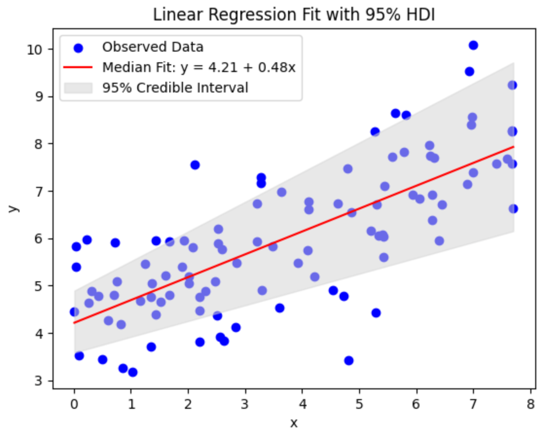
That mentioned, the posterior can nonetheless be summarized utilizing credible intervals just like the Excessive Density Interval (HDI), which incorporates all of the x% highest chance density factors.

You will need to distinction Bayesian credible intervals with frequentist confidence intervals.
- The credible interval offers a chance distribution on the doable values for the parameter i.e. the chance of the parameter assuming every worth in some interval, given the info.
- The boldness interval regards the parameter worth as mounted, and estimates as an alternative the boldness that repeated random samplings of the info would match.
Therefore the
Bayesian method lets the parameter values be fluid and takes the info at face worth, whereas the frequentist method calls for that there exists the one true parameter worth… if solely we had entry to all the info ever
Phew. Let that sink in, learn it once more till it does.
One other necessary implication of utilizing credible intervals, or in different phrases, permitting the parameter to be variable, is that the predictions we make seize this uncertainty with transparency, with a sure HDI % informing the most effective match line.

Mannequin comparability
Within the Bayesian framework, the Watanabe-Akaike Info Metric (WAIC) rating is the broadly accepted alternative for mannequin comparability. A easy rationalization of the WAIC rating is that it estimates the mannequin chance whereas regularizing for the variety of mannequin parameters. In easy phrases, it might account for overfitting. That is additionally main draw of the Bayesian framework — one does not essentially want to hold-out a mannequin validation dataset. Therefore,
Bayesian modeling gives a vital benefit when information is scarce.
The WAIC rating is a comparative measure i.e. it solely holds that means when put next throughout completely different fashions that try to elucidate the identical underlying information. Thus in apply, one can maintain including extra complexity to the mannequin so long as the WAIC will increase. If in some unspecified time in the future on this strategy of including maniacal complexity, the WAIC begins dropping, one can name it a day — any extra complexity is not going to provide an informational benefit in describing the underlying information distribution.
Conclusion
To summarize, the STAN mannequin block is solely a string. It explains to STAN what you’ll give to it (mannequin), what’s to be discovered (parameters), what you suppose is happening (mannequin), and what it ought to offer you again (generated portions).
When turned on, STAN easy turns the crank and provides its output.
The true problem lies in defining a correct mannequin (refer priors), structuring the info appropriately, asking STAN precisely what you want from it, and evaluating the sanity of its output.
As soon as we have now this half down, we are able to delve into the actual energy of STAN, the place specifying more and more difficult fashions turns into only a easy syntactical activity. In actual fact, in our subsequent tutorial we are going to do precisely this. We are going to construct upon this easy regression instance to discover Bayesian Hierarchical fashions: an trade normal, state-of-the-art, defacto… you title it. We are going to see methods to add group-level radom or mounted results into our fashions, and marvel on the ease of including complexity whereas sustaining comparability within the Bayesian framework.
Subscribe if this text helped, and to stay-tuned for extra!
References
[1] Andrew Gelman, John B. Carlin, Hal S. Stern, David B. Dunson, Aki Vehtari and Donald B. Rubin (2013). Bayesian Information Evaluation, Third Version. Chapman and Corridor/CRC.


