Your Mannequin’s MSE Is Mendacity to You III: Time Collection Diffusion

In Half I of this sequence, we began from two forecasting fashions that had the identical MSE to a few decimal locations and a really totally different degree of threat, and we traced the issue again to the loss perform itself: coaching with MSE is identical as assuming a Gaussian whose width by no means adjustments. The repair was a second output head for the variance, educated with the Gaussian unfavorable log-likelihood (NLL). In Half II we discovered that this repair quietly breaks as quickly as you forecast a couple of step forward, as a result of feeding the expected imply again into the mannequin pretends that each earlier prediction was good, and we repaired it by feeding again samples as an alternative and working many rollouts.

Each articles left one assumption untouched. A forecaster with a imply head and a variance head can let you know the place the subsequent worth of the sign can be and the way positive it’s about that, however no matter it tells you, it tells you within the type of one symmetric bell curve. For a sign that drifts and jitters this can be a completely affordable description, whereas for a sign that may leap, or change, or sit on a threshold and go both method, it isn’t, and the uncomfortable half is that the mannequin can have precisely the appropriate imply and precisely the appropriate variance and nonetheless describe a future that by no means occurs.

So if Half I was in regards to the dimension of the uncertainty and Half II was about the way it travels by means of time, this half is about its form. We’ll transfer from the easy single bell curve of Half I to a handful of bell curves, from a handful to infinitely many, and from there to a diffusion mannequin, which we are going to lastly plug into the sampled rollout of Half II with out altering the rest.

···

Diffusion for time sequence, not for pictures

Nearly each introduction to diffusion fashions I’ve learn explains them with pictures, and truly for an excellent motive, since producing pictures is what made them well-known. This text doesn’t comprise a single picture of a cat. What our diffusion mannequin generates is one quantity: the subsequent worth of a sign, given its previous.

I’ve to warn you, this can be a lengthy article, and intentionally so, as a result of I didn’t need to skip a single step of the reasoning. You don’t want to know something about diffusion fashions to comply with it. The idea comes first and the info comes final, and each determine may be reproduced with the companion pocket book.

As a result of the article is lengthy, here’s a map of it, and I’d counsel taking a look at it for a second earlier than studying on and coming again to it everytime you really feel misplaced within the particulars.

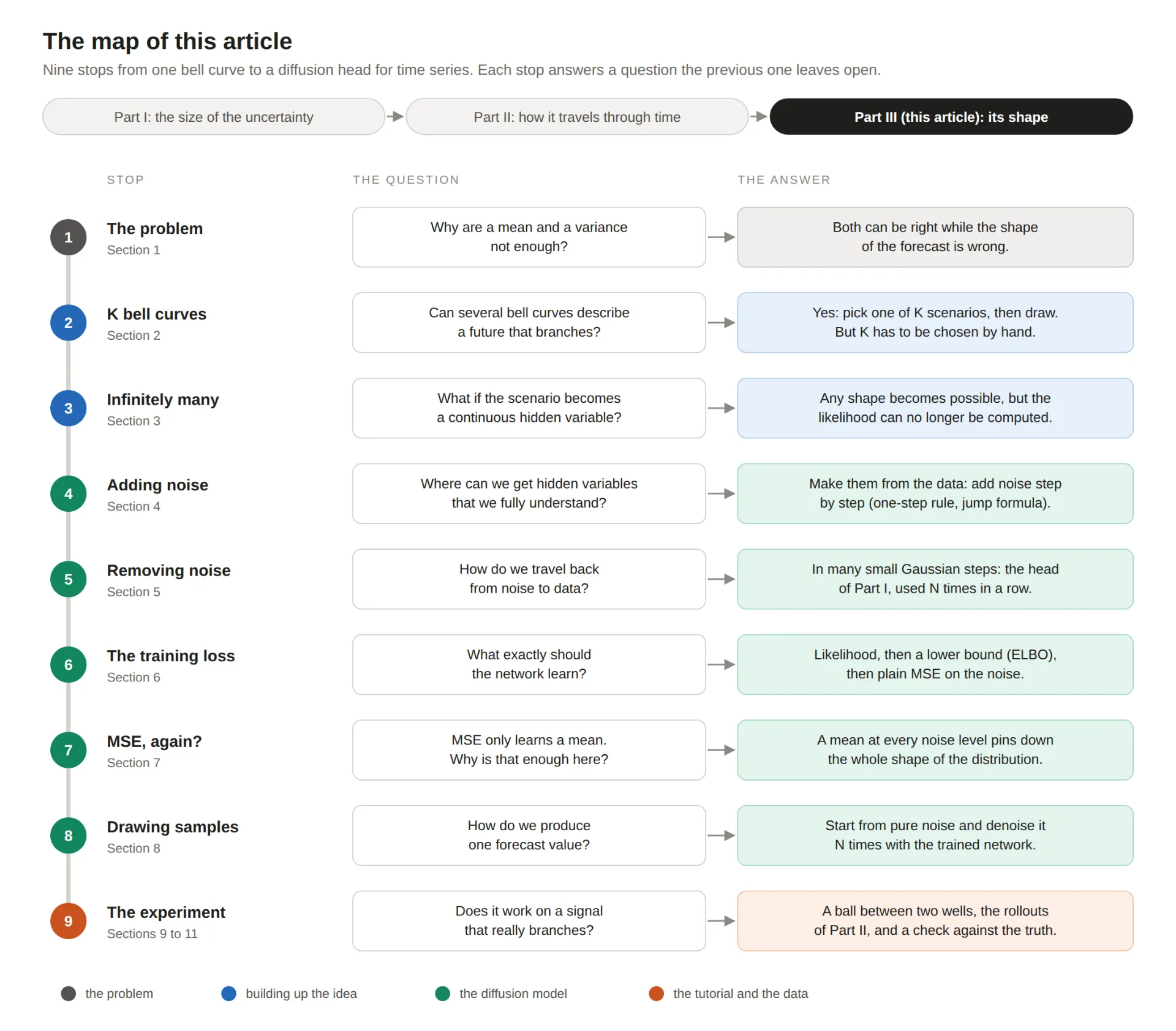
Roadmap of the article in 9 stops: the issue with a imply and a variance, mixtures of bell curves, infinitely many bell curves, including noise, eradicating noise, the coaching loss, why MSE is sufficient, drawing samples, and the forecasting experiment. Every cease lists the query it solutions and the reply in a single line.

···

1. The issue: one state of affairs, many doable futures

1.1 What a probabilistic forecast truly claims

Earlier than we will speak in regards to the form of a forecast, we ought to be exact about what a probabilistic forecast is an announcement about, as a result of that is the purpose the place the instance that follows is most simply misunderstood.

Suppose you might carry a bodily system into precisely the identical state of affairs a thousand instances, with the identical historical past and the identical current readings, and every time let it run for yet another step and write down the subsequent worth. You wouldn’t get the identical quantity a thousand instances, as a result of there are all the time influences that the previous readings don’t decide, equivalent to thermal noise, turbulence, or just issues the sensor doesn’t see. What you’d get is a group of a thousand numbers. A probabilistic forecast is an outline of that assortment. When the two-head mannequin of Half I outputs $mu = 0.5$

1.2 A state of affairs that may go two methods

Let’s now think about a system that sits on a threshold. A very good image is a ball balanced on the highest of a small hill between two valleys, however you might equally consider a valve that may both open or keep shut, or of a detector that may both preserve its lock or lose it. The ball won’t keep on the hilltop, for the reason that slightest disturbance makes it roll down, and it’ll roll both into the left valley, which I place at $-1$, or into the appropriate valley, which I place at $+1$.

If we repeat this case a thousand instances, then in roughly 5 hundred of the runs the subsequent worth $y$ finally ends up near $+1$, and within the different 5 hundred it finally ends up near $-1$, with a small scatter of about $0.1$ round every of the 2 positions. In no single run is the ball in each valleys, and in virtually no run is it nonetheless on the hilltop. The assortment of outcomes, nonetheless, consists of two separate teams, and so its histogram has two slender bumps with nothing in between.

The forecast doesn’t declare that the ball goes to each valleys; it claims that we can’t know which one, simply as with a coin earlier than it’s flipped. The trustworthy forecast for a coin is “heads or tails, fifty-fifty”, and a forecast of “half-heads” would make no sense, despite the fact that it’s the common of the 2. In the identical method, the trustworthy forecast for the ball is “the subsequent worth can be both close to $+1$ or close to $-1$, and I can’t let you know which, as a result of each are equally doubtless”.

1.3 What the two-head mannequin studies

Now let’s ask what the absolute best Gaussian head would say about this case. A Gaussian head can solely ever reply in a single format, “round $mu$, give or take $sigma$“, and when it’s educated with the Gaussian NLL, the very best reply it may well be taught is all the time the identical: $mu$ is the common of the outcomes, and $sigma$ is their typical distance from that common. A superbly educated Gaussian head mannequin subsequently studies “round 0, give or take 1“. Its single bump is centred precisely on the hilltop, which makes 0 its almost definitely worth, whereas the true ball virtually by no means finally ends up there.

For the ball, each numbers are simple to work out. Half of the outcomes are close to $+1$ and half close to$-1$, so the common is 0, proper on the hilltop. Each consequence lies about 1 away from 0, so $sigma$ is about 1. (Extra exactly, $sigma^2 = 1^2 + 0.1^2 = 1.01$

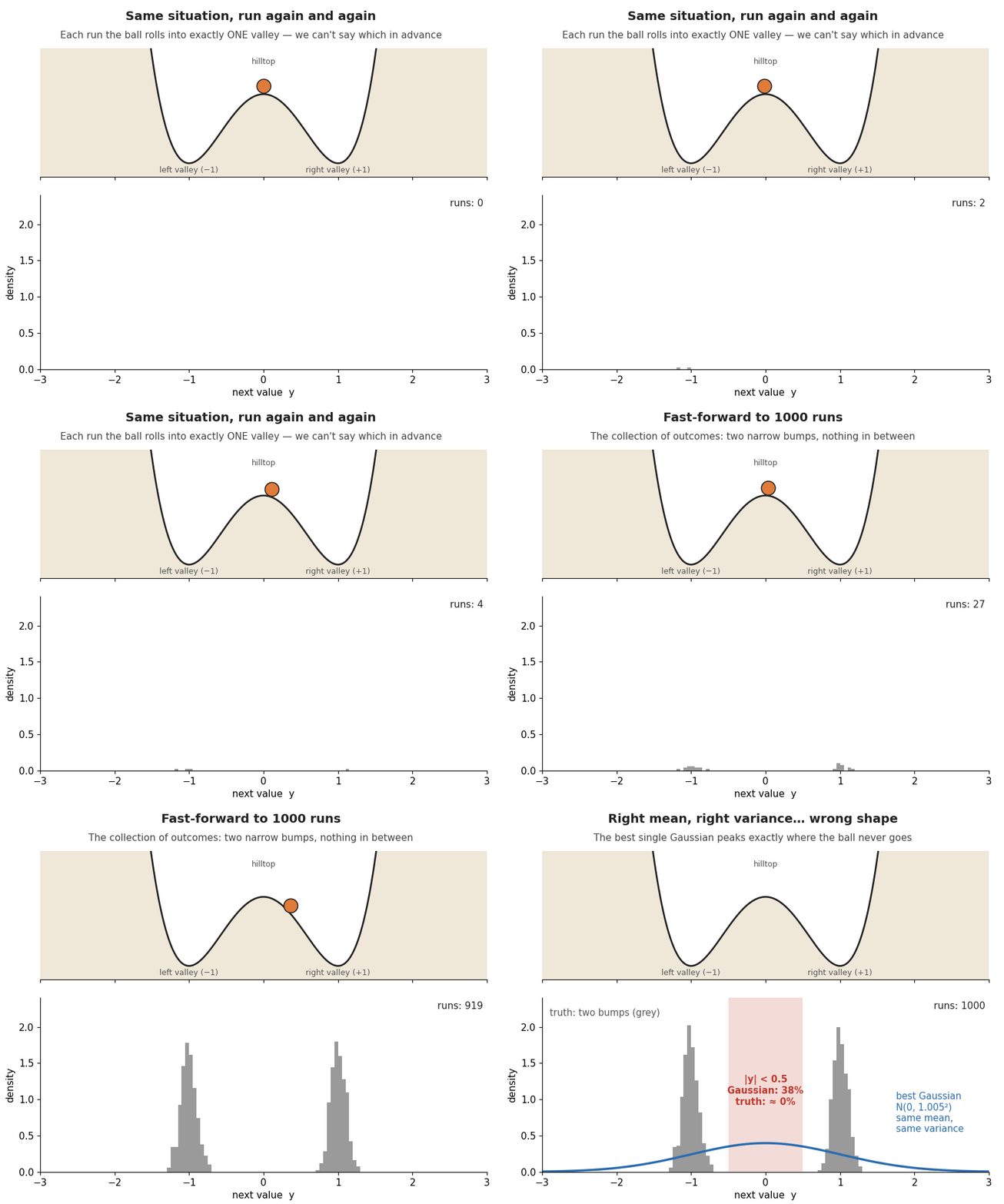
Animated thought experiment for probabilistic forecasting. The identical state of affairs is run many times, and every time the ball rolls into precisely considered one of two valleys, so the outcomes kind two slender bumps at minus one and plus one. One of the best single Gaussian has the identical imply and variance, but it peaks on the hilltop and places about 38% of its chance the place the ball by no means goes.

The imply is right and the variance is right, so nothing went mistaken throughout coaching, and nonetheless the forecast is mistaken in the one sense that issues, as a result of the worth it considers most possible is the one place the place the ball will definitely not be. In Half I the 2 fashions differed in a quantity that MSE couldn’t see, specifically the variance, and right here the forecast and the reality differ in one thing that even the imply and the variance collectively can’t see.

1.4 Why this issues much more in a rollout

The injury turns into worse as soon as we bear in mind Half II. If we pattern from this Gaussian and feed the samples again into the mannequin, which is precisely what a sampled rollout does, then roughly 38 % ($frac{1}{2} sigma$

···

2. First step past the bell curve: Ok bell curves

2.1 The concept

If one bell curve can’t describe two bumps, the most pure restore is to make use of two bell curves, or extra typically $Ok$ of them, and to let the mannequin say how a lot weight each ought to get. That is known as a combination of Gaussians, and a forecaster that outputs its parameters is named a combination density community. Its forecast for the subsequent worth is a weighted sum of bell curves:

$underbrace{p(y mid textual content{context})}_{textual content{forecast}} ;=; sum_{okay=1}^{Ok} overbrace{textcolor{#E07B39}{pi_k}}^{textual content{weight}}; overbrace{mathcal{N}huge(y mid underbrace{textcolor{#2B6CB0}{mu_k}}_{textual content{centre}},, underbrace{textcolor{#2F9E5B}{sigma_k^2}}_{textual content{width}}huge)}^{textual content{bell curve } okay}$

Each one of many $Ok$ elements has three numbers. The weight $pi_k$

2.2 How a mix produces a pattern, and the hidden variable inside it

The way in which a pattern is drawn from a mix deserves a detailed look, as a result of it incorporates the seed of every little thing that follows. Drawing a pattern takes two phases. Within the first stage we select one of many $Ok$ elements at random, the place part $okay$ is chosen with chance $pi_k$

$okay sim textual content{Categorical}(pi_1, dots, pi_K), qquad y = mu_k + sigma_k,varepsilon, quad varepsilon sim mathcal{N}(0, 1)$

For the ball, that is flip a coin to determine which valley, then add just a little scatter. The index $okay$ is a amount that the mannequin makes use of internally and that by no means seems within the information, since our sensor data the place of the ball and never a label that claims which situation it belongs to. Such a amount is named a hidden variable (or latent variable), and with it the combination may be written in a kind that we are going to meet many times, the chance of every situation multiplied by a easy bell curve for that situation:

$p(y) = sum_{okay=1}^{Ok} underbrace{p(okay)}_{textual content{how doubtless is situation } okay} ;underbrace{p(y mid okay)}_{textual content{a easy bell curve}}$

This method carries the central lesson of this part: an advanced distribution may be constructed from easy bell curves, supplied {that a} hidden variable decides which bell curve is used. Every bit is so simple as the Gaussian head of Half I, and all of the richness comes from the hidden alternative.

2.3 The place a handful of bell curves stops being sufficient

A combination has three weaknesses, and they’re value stating clearly as a result of the subsequent part addresses exactly these.

• The primary is that the quantity $Ok$ must be chosen prematurely and by hand. Two elements are proper for the ball on the hilltop, however, typically, for a sensible sign you have no idea prematurely what number of elements exist.

• The second is that many shapes should not “just a few bumps” in any respect. A distribution with a protracted tail on one facet, a ridge, or a bump whose place varies constantly can solely be approximated by inserting a fantastic many slender elements facet by facet.

• The third is extra refined and considerations coaching. Since we by no means observe which part produced a given information level, the chance of that information level has so as to add up the contributions of all elements, which is the sum within the method above. With $Ok = 2$

···

3. Second step: infinitely many bell curves

3.1 From a listing of situations to a continuum

If the difficulty with a mix is that $Ok$ is a small quantity we’ve got to decide on, the boldest method out is to cease counting. As an alternative of a hidden index $okay$ that takes considered one of $Ok$ values, we use a hidden variable $z$ that could be a steady quantity, and we draw it from the best distribution there may be, a regular Gaussian. As an alternative of a listing of $Ok$ means $mu_1, dots, mu_K$

$underbrace{p(y)}_{textual content{forecast}} ;=;underbrace{intoverbrace{textcolor{#E07B39}{p(z)}}^{textual content{weight}}; overbrace{mathcal{N}huge(y mid underbrace{textcolor{#2B6CB0}{mu(z)}}_{textual content{centre}},, underbrace{textcolor{#2F9E5B}{sigma^2}}_{textual content{width}}huge)}^{textual content{bell curve for this } z} ; dz}_{textual content{add up one bell curve for each } z}, qquad textcolor{#E07B39}{p(z)} = underbrace{mathcal{N}(z mid 0, 1)}_{textual content{plain bell curve}}$

It helps to place the 2 formulation facet by facet and to see that each ingredient of the combination has merely been changed by its steady counterpart:

Drawing a pattern works precisely as earlier than, in two phases, the place we first draw the hidden variable after which draw from the bell curve it selects:

$z sim mathcal{N}(0, 1), qquad y = mu(z) + sigma,varepsilon, quad varepsilon sim mathcal{N}(0, 1)$

3.2 An instance you may compute by hand

To see how a lot freedom this provides, take the perform $mu(z) = tanh(8z)$

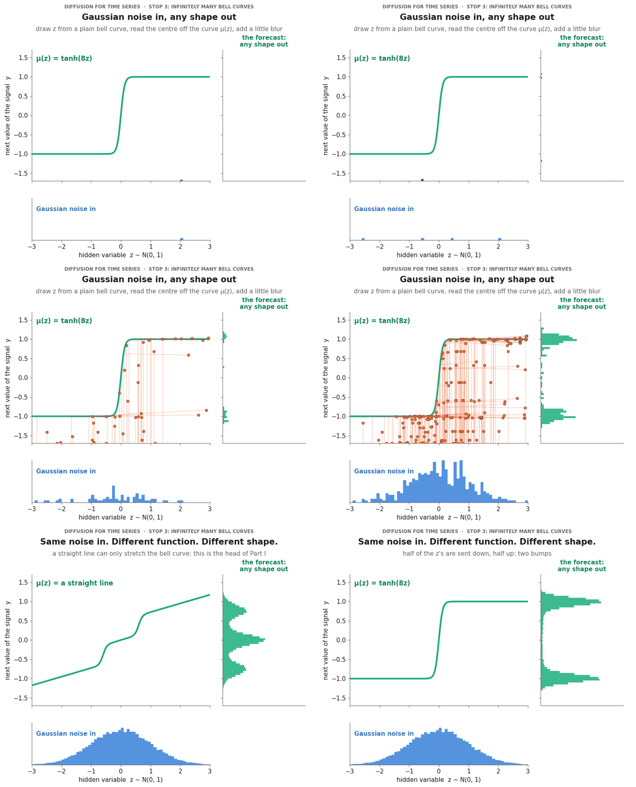
Animated demonstration of a steady combination. Values drawn from a regular Gaussian are mapped by means of a perform and blurred barely, and the output histogram builds up on the appropriate. When the perform adjustments, the forecast distribution adjustments with it: a straight line provides a bell curve, an S-curve provides two bumps, a staircase provides three bumps, and an exponential provides a protracted tail.

If $mu$ is a neural community $mu_theta$

3.3 The worth: the chance can not be computed

To date we’ve got solely seen how such a mannequin generates samples as soon as the perform $mu_theta$

With a mix of $Ok$ elements, the corresponding amount was a sum of $Ok$ phrases, and we might merely compute it. Right here the sum has grow to be an integral over all doable values of the hidden variable, with a neural community inside it. Such an integral has no closed kind, which signifies that there is no such thing as a method we might write down and consider precisely.

The mannequin is highly effective sufficient, however on this kind it is rather laborious to coach. (Variational autoencoders practice precisely this sort of mannequin by studying a second community that guesses $z$ from $y$; diffusion fashions take a special route, which is the topic of the remainder of this text.)

3.4 The way in which out: construct the hidden variables ourselves

Diffusion fashions resolve this problem with two concepts which might be each easy, and that I would really like you to hold by means of the remainder of the article.

The primary thought is to cease treating the hidden variable as a thriller. Within the steady combination, the hidden variable was an summary quantity whose relation to the info needed to be found. A diffusion mannequin as an alternative constructs its hidden variables straight from the info, by a set and totally identified recipe: it takes the info worth and provides noise to it. The hidden variable is then nothing greater than a loud copy of the info, and for each coaching instance we all know precisely which hidden variables belong to it, as a result of we made them ourselves.

The second thought is to exchange one massive leap by many small steps. Within the steady combination, a single perform $mu(z)$ needed to flip pure noise into information in a single go, deciding every little thing directly. A diffusion mannequin as an alternative provides noise step by step, creating a series of copies that vary from virtually clear to pure noise, and learns to stroll again one small step at a time. Consider a movie of ink spreading in water: guessing the primary body from the final one is hopeless, however guessing body 99 from body 100 is straightforward, as a result of the 2 frames are virtually an identical. Every small step again is so easy that one bell curve describes it nicely, which is precisely what the Gaussian head of Half I can do. And since we made the noisy copies ourselves (the primary thought), we all the time know which copy belongs to which information level, so each step may be educated straight.

Collectively they provide us two paired processes. The ahead course of provides noise to a clear worth step-by-step till solely noise is left, and entails no studying in any respect (Part 4). The reverse course of is a neural community that removes just a little noise at every step (Part 5), and we must work out what it ought to be educated to do (Sections 6 and seven) and the way it produces a forecast worth (Part 8).

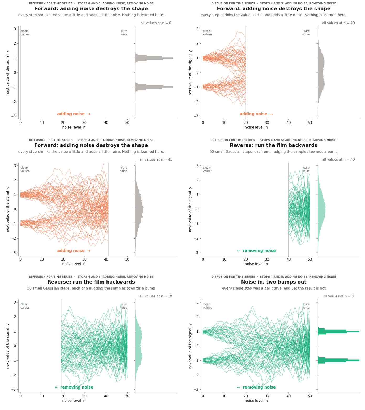
Animated view of each diffusion processes. Going ahead, including noise step-by-step melts the two-bump distribution right into a plain bell curve. Stepping into reverse, fifty small Gaussian steps flip the bell curve again into two bumps. The reverse steps use the precise finest guess of the clear worth, with no neural community concerned.

3.5 A phrase on notation

From right here on there are two totally different sorts of “time” in play, and holding them aside avoids a lot of the confusion round diffusion fashions for time sequence. On this sequence, $t$ has all the time been the time index of the sign and $T$ the context size, so I’ll preserve these and use the letter $n$ for the noise degree. Most diffusion papers name the noise degree $t$ and the variety of ranges $T$, which you must consider in the event you learn them alongside this text.

Two remarks will preserve the subsequent sections mild. Since we forecast one studying at a time, the amount being noised and denoised is a single quantity, the subsequent worth of the sign (for vectors, equivalent to pictures, each method holds in the identical kind for every part). And every little thing in Sections 4 to eight occurs for a given context: the forecast distribution is all the time the distribution of the subsequent worth given the previous, however I depart the context out of the formulation till Part 9, the place it comes again as an additional enter of the community.

···

4. The ahead course of: including noise

Purpose of this part. We would like a recipe that step by step turns a clear worth $y_0$

4.1 Two issues to learn about Gaussians

A Gaussian distribution $mathcal{N}(mu, sigma^2)$

$X = mu + sigma,varepsilon, qquad varepsilon sim mathcal{N}(0, 1)$

That is known as reparameterisation, and it’s precisely how the Gaussian head of Half I attracts a pattern. It appears like a small trick, however it’s the engine of every little thing on this part, as a result of it lets us write each noising step as an extraordinary equation as an alternative of as a chance distribution. The notation $mathcal{N}(X mid mu, sigma^2)$

4.2 One small step

We begin with a clear worth $y_0$

$underbrace{q(y_n mid y_{n-1})}_{textual content{one noising step}}= mathcal{N}huge(y_n ;huge|; underbrace{textcolor{#2B6CB0}{sqrt{1 – beta_n};y_{n-1}}}_{textual content{centre: outdated worth, shrunk}},; underbrace{textcolor{#2F9E5B}{beta_n}}_{textual content{width: noise added}}huge)$

and in reparameterised kind, which is the shape we truly use in code,

$boxed{,y_n = underbrace{textcolor{#2B6CB0}{sqrt{1 – beta_n};y_{n-1}}}_{textual content{shrink the outdated worth just a little}} ;+; underbrace{textcolor{#2F9E5B}{sqrt{beta_n};varepsilon_n}}_{textual content{add just a little contemporary noise}}, qquad varepsilon_n sim mathcal{N}(0, 1),}$

The letter$q$ is used for this fastened ahead course of, and we are going to use $p_theta$

What’s $beta_n$

4.3 Why $sqrt{1 – beta_n}$

It is a design alternative, however it’s a principled one, and seeing the place it comes from takes just one objective and two primary info about random numbers.

The objective: preserve the variance equal to 1 at each step. Era will begin from a regular Gaussian, $mathcal{N}(0, 1)$, so the ahead course of should finish precisely there, as a result of in any other case the community can be educated on one form of enter and used on one other. The only option to assure that is to standardise the info to variance 1 and to maintain the variance at 1 at each single step, which additionally retains the inputs of the community on the identical scale at each noise degree.

• Rule 1: scaling a random quantity squares the consider its variance. If $X$ has variance $sigma^2$ and we multiply it by a relentless $a$, then $mathrm{Var}(aX) = a^2,mathrm{Var}(X)$

• Rule 2: the variances of impartial random numbers add up. If $X$ and $Y$ are impartial, then $mathrm{Var}(X + Y) = mathrm{Var}(X) + mathrm{Var}(Y)$

Constructing the method from the objective. Let’s combine the earlier worth with contemporary noise utilizing two unknown constants $a$ and $b$,

$y_n = a,y_{n-1} + b,varepsilon_n$

and compute the variance of the end result. Since $y_{n-1}$

$mathrm{Var}(y_n) = a^2,underbrace{mathrm{Var}(y_{n-1})}_{=,1} + b^2,underbrace{mathrm{Var}(varepsilon_n)}_{=,1} = a^2 + b^2$

Variance preservation subsequently requires $a^2 + b^2 = 1$

$a = sqrt{1 – beta_n}, qquad b = sqrt{beta_n}$

so the sq. roots should not arbitrary in any respect, since they’re the one constructive answer of $a^2 + b^2 = 1$

Verifying that it really works. Plugging again in, $mathrm{Var}(y_n) = (sqrt{1 – beta_n})^2 + (sqrt{beta_n})^2 = (1 – beta_n) + beta_n = 1$

What goes mistaken with out the sq. roots? Suppose we had naively used $y_n = (1 – beta_n),y_{n-1} + beta_n,varepsilon_n$

4.4 The leap method: from the clear worth to any noise degree in a single shot

Coaching would require noisy variations $y_n$

Step 0: the Gaussian addition rule. Earlier than doing any algebra, we’d like one reality that may do all of the heavy lifting. If $A sim mathcal{N}(0, sigma_1^2)$

$A + B sim mathcal{N}(0,; sigma_1^2 + sigma_2^2)$

The variance half is Rule 2 from above. The extra assertion, that the sum of two impartial Gaussians is once more a Gaussian, is a regular results of chance idea. Collectively they are saying that two impartial Gaussian noises can all the time get replaced by a single Gaussian noise whose variance is the sum of the 2 variances.

Step 1: shorter notation. Let $alpha_n = 1 – beta_n$

$y_n = sqrt{alpha_n};y_{n-1} + sqrt{1 – alpha_n};varepsilon_n$

Step 2: increasing two steps. Let’s write out two consecutive steps to see the sample. Step one goes from $y_0$

$y_1 = sqrt{alpha_1};y_0 + sqrt{1 – alpha_1};varepsilon_1$

The second step goes from $y_1$

$y_2 = sqrt{alpha_2};y_1 + sqrt{1 – alpha_2};varepsilon_2= sqrt{alpha_2},Large(sqrt{alpha_1};y_0 + sqrt{1 – alpha_1};varepsilon_1Big) + sqrt{1 – alpha_2};varepsilon_2$

$y_2 = underbrace{sqrt{alpha_1 alpha_2};y_0}_{textual content{sign}} ;+; underbrace{sqrt{alpha_2 (1 – alpha_1)};varepsilon_1 + sqrt{1 – alpha_2};varepsilon_2}_{textual content{two noise phrases}}$

We now have one clear sign time period and two separate noise phrases, and the subsequent step is to merge the latter.

Step 3: merging the 2 noise phrases. That is the place the addition rule of Step 0 does its work. The noises$varepsilon_1$

$alpha_2 (1 – alpha_1) + (1 – alpha_2) = alpha_2 – alpha_1 alpha_2 + 1 – alpha_2 = 1 – alpha_1 alpha_2$

The 2 noise phrases subsequently collapse into one,

$sqrt{alpha_2 (1 – alpha_1)};varepsilon_1 + sqrt{1 – alpha_2};varepsilon_2 ;=; sqrt{1 – alpha_1 alpha_2};barvarepsilon, qquad barvarepsilon sim mathcal{N}(0, 1)$

the place the equality signifies that each side have the identical distribution, and substituting again provides

$y_2 = sqrt{alpha_1 alpha_2};y_0 + sqrt{1 – alpha_1 alpha_2};barvarepsilon$

Step 4: the overall method. The sample is now seen, and the identical arithmetic extends to any variety of steps: the sign is multiplied by the sq. root of the product of all of the $alpha$‘s, and the mixed noise has variance one minus that product. If we outline the working product

$baralpha_n = alpha_1 ,alpha_2 cdots alpha_n = prod_{s=1}^{n} alpha_s$

then for any noise degree $n$ all of the intermediate noise phrases collapse right into a single one, and we acquire the leap method:

$boxed{,y_n = underbrace{textcolor{#2B6CB0}{sqrt{baralpha_n};y_0}}_{textual content{what’s left of the clear worth}} ;+; underbrace{textcolor{#2F9E5B}{sqrt{1 – baralpha_n};varepsilon}}_{textual content{all of the noise of } n textual content{ steps, in a single draw}}, qquad varepsilon sim mathcal{N}(0, 1),}$

Written as a chance distribution, this says the identical factor:

$q(y_n mid y_0) = mathcal{N}huge(y_n mid underbrace{textcolor{#2B6CB0}{sqrt{baralpha_n};y_0}}_{textual content{centre}},; underbrace{textcolor{#2F9E5B}{1 – baralpha_n}}_{textual content{width}}huge)$

You may learn it as a recipe, which says that we preserve a fraction $sqrt{baralpha_n}$

The payoff. We by no means should loop by means of the noising steps throughout coaching. We choose a noise degree, draw a single $varepsilon$, and compute $y_n$

4.5 The noise schedule

We nonetheless have to decide on the numbers $beta_1, dots, beta_N$

The schedule decides how our fastened variety of steps is spent. If the sign disappears too slowly, the chain by no means reaches pure noise, and technology would then begin from inputs the community has by no means seen. If it disappears too shortly, a lot of the steps are wasted on turning noise into extra noise, whereas the attention-grabbing half, the place the bumps merge, is squeezed into just a few massive steps, and huge steps are precisely what the reverse course of can’t deal with (Part 5). A very good schedule lets the sign fade at a gradual tempo, so that each step does an identical, small quantity of labor.

One possibility is to decide on the$beta_n$

$beta_n = 1 – alpha_n = 1 – frac{baralpha_n}{baralpha_{n-1}}$

A preferred curve of this sort is the cosine schedule,

$baralpha_n = frac{f(n)}{f(0)}, qquad f(n) = cos^2!left(frac{pi}{2} cdot frac{n/N + 0.008}{1 + 0.008}proper)$

by which the division by $f(0)$makes positive that $baralpha_0 = 1$

The linear schedule, run over solely 50 steps, nonetheless leaves 60 % of the sign on the finish, so it fails the too gradual take a look at, and even with 1,000 steps it’s fairly quick, since a couple of third of its steps occur when lower than 1 % of the sign is left. The cosine curve falls gently and evenly, which is why it was proposed and why the companion pocket book makes use of it with $N = 50$

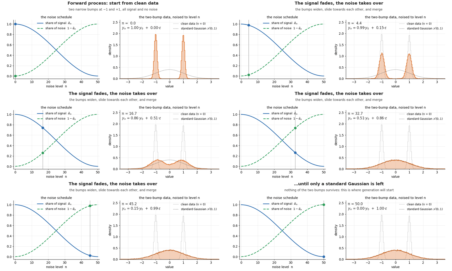
Animated diffusion ahead course of: a cosine noise schedule shrinks the sign and provides noise step-by-step, turning a two-peaked distribution into a regular Gaussian.

···

5. The reverse course of: eradicating noise

5.1 One huge leap is difficult, one small step is straightforward

Suppose someone arms you pure noise $y_N$

Now suppose as an alternative that you’re handed $y_n$

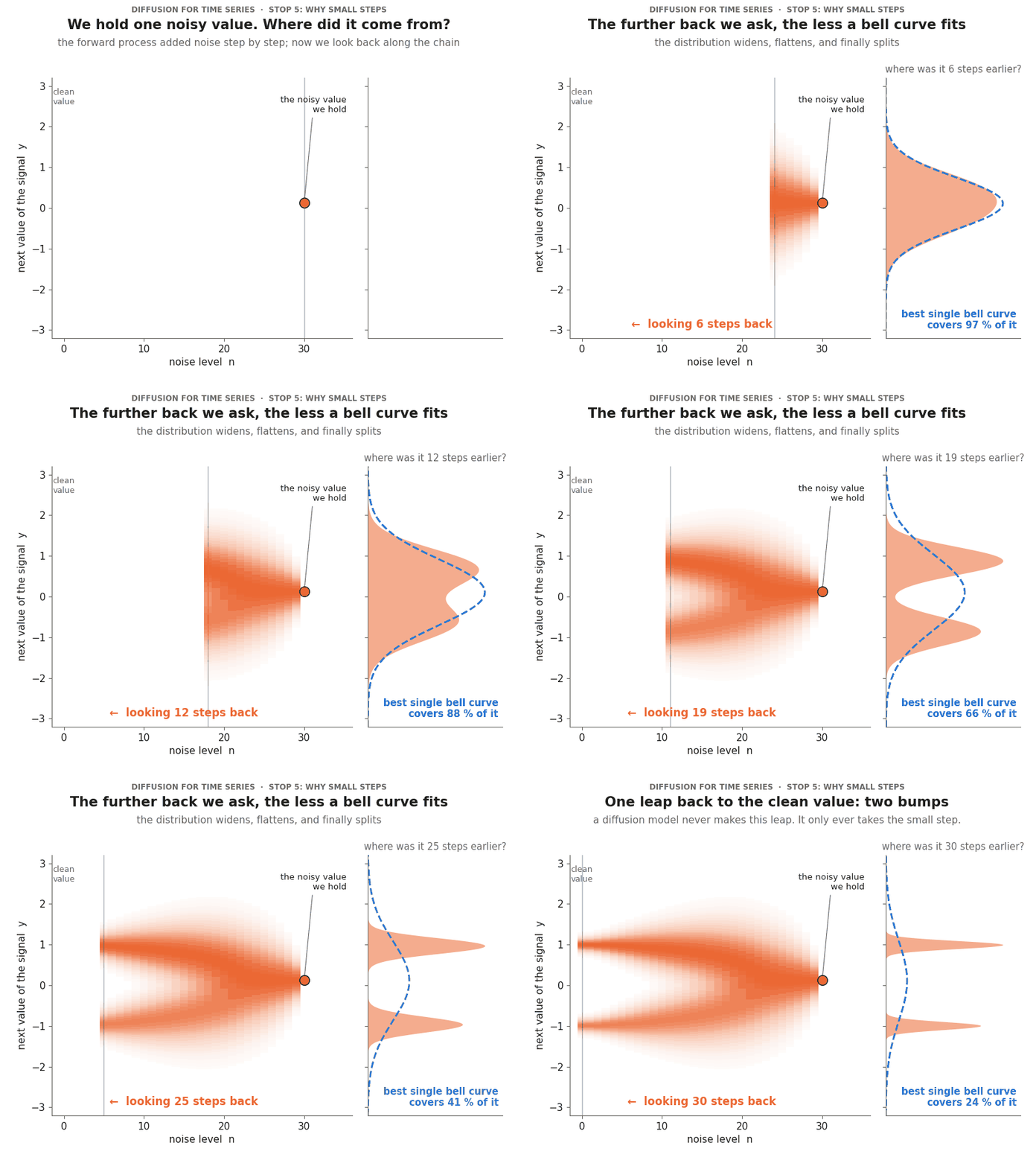
Animated rationalization of why diffusion fashions use many small steps. Ranging from one noisy worth at noise degree 30, the animation reveals the place that worth was one step earlier, two steps earlier, and so forth. One step again the reply is a slender bell curve {that a} single Gaussian covers virtually fully; thirty steps again it has break up into two bumps, of which a single Gaussian covers lower than 1 / 4.

That is the important thing statement of the entire technique: when every ahead step provides solely just a little noise, every reverse step is roughly Gaussian, despite the fact that the distribution of the info shouldn’t be.

5.2 Every reverse step is a Gaussian head

We subsequently mannequin each reverse step as a Gaussian whose imply is predicted by a neural community:

$underbrace{p_theta(y_{n-1} mid y_n)}_{textual content{one denoising step}}= mathcal{N}huge(y_{n-1} mid underbrace{textcolor{#2B6CB0}{mu_theta(y_n, n)}}_{textual content{centre: realized}},; underbrace{textcolor{#2F9E5B}{sigma_n^2}}_{textual content{width: fastened}}huge)$

If this appears acquainted, it ought to, as a result of it’s the two-head mannequin of Half I with two small adjustments:

• The variance is fastened, not realized. The community solely predicts the imply; the width of every step is about by the noise schedule.

• It’s used $N$ instances in a row, not as soon as. Every name removes just a little noise, taking the noisy worth $y_n$

A single community serves all of the steps, and it’s advised at which noise degree it’s working, in order that it may well behave otherwise when it’s eradicating heavy noise and when it’s sprucing the final particulars.

5.3 The place does the form come from?

Since each single step is Gaussian, you might marvel the place the non-Gaussian form comes from, and there are two methods of seeing it that tie this part to the sooner ones.

The primary method is to take a look at the final step of the chain. The ultimate worth $y_0$

$p_theta(y_0) = int p_theta(y_1);mathcal{N}huge(y_0 mid mu_theta(y_1, 1),; sigma_1^2big);dy_1$

If you happen to examine this with the continual combination (Part 3), you will note that it’s the identical method, with the noisy worth $y_1$

The second method is to take a look at the chain as a complete. Every step strikes the pattern by a small quantity in a route chosen by a nonlinear perform $mu_theta$

···

6. Coaching: what ought to the community be taught?

Purpose of this part. We need to practice a mannequin $varepsilon_theta(y_n, n)$

Step 1: why cannot we simply invert the ahead course of?

The leap method advised us learn how to go from a clear worth to a loud one in a single shot:

$y_n = sqrt{baralpha_n};y_0 + sqrt{1 – baralpha_n};varepsilon$

Naively, one may suppose that that is all we’d like, since we will merely rearrange it for $y_0$

$underbrace{y_0}_{textual content{what we wish}} = frac{overbrace{y_n}^{textual content{what we maintain}} – sqrt{1 – baralpha_n};overbrace{textcolor{#2F9E5B}{varepsilon}}^{textual content{unknown!}}}{sqrt{baralpha_n}}$

The issue is that $varepsilon$ is gone. After we ran the ahead course of we drew $varepsilon$ at random and combined it into $y_n$

That is precisely why we’d like a neural community: to estimate $varepsilon$ from the noisy worth alone. If we will make an excellent guess of what $varepsilon$ was, the rearranged method provides us a guess of $y_0$

The derivation that follows is the toughest a part of the article, so right here is its vacation spot and its essential strikes earlier than the primary equation. (1) We can’t compute how possible the info is below the mannequin, as a result of that might require each doable path of noisy values. (2) So we rating the mannequin solely on paths that we generate ourselves, which supplies a decrease sure on that chance. (3) This rating splits into one comparability per noise degree, between the step of the community and a super step that is aware of the clear worth. (4) Each steps are bell curves of the identical width, so every comparability is a squared error, and after a change of variables it’s a squared error on the noise.

Step 2: what ought to the community truly optimise?

The objective. As in all places on this sequence, we wish the mannequin to present a excessive chance to the info we truly noticed, so we need to maximise $log p_theta(y_0)$

The issue. The mannequin by no means produces $y_0$

$p_theta(y_0, y_1, dots, y_N) = p(y_N)prod_{n=1}^{N} p_theta(y_{n-1} mid y_n)$

In phrases, that is the chance of ranging from this specific noise (which is simply a regular Gaussian) multiplied by the chance of every denoising step. To acquire the chance of $y_0$

$p_theta(y_0) = int p_theta(y_0, y_1, dots, y_N);dy_1 cdots dy_N$

Consider a metropolis map. “How doubtless is that this one route?” is a simple query, because you multiply the possibilities of every flip, whereas “how doubtless am I to finish up at this deal with, by any route?” means summing over all routes. With $N = 50$

The answer: rating solely the paths we make ourselves. We usher in our personal ahead course of, $q(y_{1:N} mid y_0)$

(a) Multiply by 1. We multiply and divide by $q$, which adjustments nothing:

$p_theta(y_0) = int q(y_{1:N} mid y_0);frac{p_theta(y_0, y_{1:N})}{q(y_{1:N} mid y_0)};dy_{1:N}$

(b) Recognise a median. An integral by which one thing is weighted by a distribution $q$ is a median over samples from $q$:

$p_theta(y_0) = mathbb{E}_q!left[frac{p_theta(y_0, y_{1:N})}{q(y_{1:N} mid y_0)}right]$

(c) Take the logarithm of each side, for the reason that log-likelihood is what we’re after.

(d) Transfer the logarithm inside the common (Jensen’s inequality). The logarithm bends downwards, so the logarithm of a median is all the time a minimum of as massive as the common of the logarithms. For the 2 numbers 1 and 100, for instance, the logarithm of their common is $log 50.5 approx 3.9$

$underbrace{log p_theta(y_0)}_{textual content{what we wish (can’t compute)}} ;ge; underbrace{mathbb{E}_q}_{substack{textual content{common over noise}textual content{paths we generate}}}!left[log frac{overbrace{p_theta(y_0, y_{1:N})}^{text{model: denoise along the path}}} {underbrace{q(y_{1:N} mid y_0)}_{text{us: noise along the path}}}right] = textual content{ELBO}$

The appropriate-hand facet is named the proof decrease sure (“proof” is one other identify for the chance of the info). Not like the left-hand facet, it may be computed: we generate noise paths ourselves and consider two issues we all know, $q$ (how we add noise) and $p_theta$

Step 3: how does the ELBO grow to be MSE?

A. One comparability per noise degree. The ratio contained in the ELBO is a product of $N$ backward steps (the mannequin) divided by a product of $N$ ahead steps (the noising). To check them step-by-step, we flip each ahead step round with Bayes’ theorem, in order that it factors backwards too. We’re allowed to situation every little thing on $y_0$

$q(y_1 mid y_0);q(y_2 mid y_1) ;=; q(y_1 mid y_0)cdotfrac{q(y_1 mid y_2, y_0);q(y_2 mid y_0)}{q(y_1 mid y_0)} ;=; q(y_2 mid y_0);q(y_1 mid y_2, y_0)$

The issue $q(y_1 mid y_0)$

$-text{ELBO} = sum_{n=2}^{N} mathbb{E}_qBig[mathrm{KL}big(underbrace{q(y_{n-1} mid y_n, y_0)}_{text{the cheat sheet}};big|;underbrace{p_theta(y_{n-1} mid y_n)}_{text{the network}}big)Big] ;+; textual content{two finish phrases}$

The image $mathrm{KL}$ stands for the Kullback-Leibler divergence, which measures how totally different two distributions are: it’s zero once they agree and constructive in any other case. Every time period compares two solutions to the identical query, “the place was the worth one step earlier?”. The primary reply, $q(y_{n-1} mid y_n, y_0)$

B. The cheat sheet is a bell curve. Two witnesses converse in regards to the unknown $y_{n-1}$

$q(y_{n-1} mid y_n, y_0) = mathcal{N}huge(y_{n-1} mid tildemu_n,; tildesigma_n^2big), qquad tildemu_n = a_n,underbrace{y_n}_{textual content{the place we are actually}} ;+; c_n,underbrace{y_0}_{textual content{the place we got here from}}$

The weights $a_n$

C. Equal widths flip the KL divergence right into a squared error. We make the step of the community a bell curve with the identical width $tildesigma_n^2$

$mu_theta = a_n, y_n + c_n, hat y_0$

For 2 bell curves of equal width, the KL divergence is just the squared distance between their centres, divided by twice the variance. The elements $a_n y_n$

$mathrm{KL} = frac{(tildemu_n – mu_theta)^2}{2tildesigma_n^2} = underbrace{frac{c_n^2}{2tildesigma_n^2}}_{textual content{fastened weight}}; underbrace{huge(y_0 – hat y_0big)^2}_{textual content{squared error on the clear worth}}$

Readers of Half I will recognise this second, as a result of it’s the central assertion of that article in a brand new place: below a Gaussian with a set width, most chances are a squared error.

D. Clear worth or noise: the identical factor. By the leap method, figuring out $y_n$

$y_0 = frac{y_n – sqrt{1-baralpha_n};varepsilon}{sqrt{baralpha_n}},qquad hat y_0 = frac{y_n – sqrt{1-baralpha_n};varepsilon_theta}{sqrt{baralpha_n}} qquadLongrightarrowqquad y_0 – hat y_0 = -sqrt{frac{1-baralpha_n}{baralpha_n}};huge(varepsilon – varepsilon_thetabig)$

Each time period of the ELBO is subsequently a weight, which relies upon solely on the noise degree, multiplied by $(varepsilon – varepsilon_theta)^2$

$boxed{,L_{textual content{easy}} = mathbb{E}_{,y_0,; n,; varepsilon}Large[big(underbrace{textcolor{#2F9E5B}{varepsilon}}_{text{true noise}} – underbrace{varepsilon_theta(y_n, n)}_{text{networktextquoteright s guess}}big)^2Big], qquad y_n = textcolor{#2B6CB0}{sqrt{baralpha_n};y_0} + textcolor{#2F9E5B}{sqrt{1 – baralpha_n};varepsilon},}$

That’s plain MSE. (Strictly talking, as soon as the weights are dropped it’s not precisely the ELBO however a re-weighted model of it.)

Step 4: the coaching loop, placing all of it collectively

Now that we’ve got the loss perform, coaching is easy, and one coaching step consists of the next eight actions:

1. Pattern a clear worth $y_0$

2. Pattern a random noise degree $n$ uniformly from ${1, dots, N}$

3. Pattern a random noise $varepsilon sim mathcal{N}(0, 1)$

4. Compute the noisy worth in a single shot with the leap method: $y_n = sqrt{baralpha_n};y_0 + sqrt{1 – baralpha_n};varepsilon$

5. Ahead go: feed $(y_n, n)$

6. Community output: the expected noise $varepsilon_theta(y_n, n)$

7. Compute the loss: $huge(varepsilon – varepsilon_theta(y_n, n)huge)^2$

8. Backpropagate and replace the weights of the community.

That is repeated for a lot of mini-batches, and the community step by step learns to denoise at each noise degree. Discover that no chain is run throughout coaching and that there is no such thing as a sampling loop, since each coaching step is one extraordinary ahead go adopted by one extraordinary backward go. Determine 7 reveals this loop at work on the two-bump information.

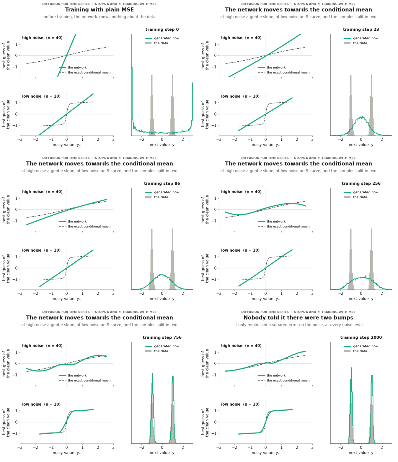
Animated coaching run of a small denoising community on two-bump information. Left: the community’s finest guess of the clear worth at a excessive and at a low noise degree, subsequent to the precise conditional imply proven dashed. Proper: the samples the community generates at that second. After 2,000 coaching steps with a imply squared error loss on the noise, the guesses match the precise curves and the samples kind two bumps.

···

7. Wait, MSE once more? Wasn’t that the liar?

Now we have arrived at a wierd place. This sequence started by displaying that MSE solely learns the conditional imply and subsequently can’t specific uncertainty, and now we’re coaching a mannequin with MSE and claiming that it captures not solely the uncertainty however its whole form. Each statements are true, and reconciling them is the bridge between this text and the primary one.

7.1 What MSE learns, right here as in all places

If you happen to predict a random amount $Y$ with a single quantity $m$ and you might be penalised by $mathbb{E}[(Y – m)^2]$

$hat{y}_0(y_n, n) = mathbb{E}huge[,y_0 mid y_n,, n,big]$

The dashed curves of Determine 7 are precisely this amount. The diffusion community is subsequently nonetheless a conditional-mean predictor, precisely just like the MSE mannequin of Half I. What has modified is the query it’s requested. The mannequin of Half I was requested one query, specifically what the long run is on common.

The diffusion community is requested a complete household of questions, one for each noise degree and each doable noisy worth: “if the clear worth had been noised this a lot and now regarded like this, what was it on common?” A single imply doesn’t decide a distribution, however the entire household of means throughout all noise ranges does. Strictly, this holds within the restrict of infinitely many, infinitely small steps; with a finite variety of steps the form is reproduced solely roughly, and the approximation improves because the steps get smaller.

7.2 Two instances we will compute by hand

The 2-bump instance lets us see this with formulation. Suppose first that the clear worth actually is Gaussian,$y_0 sim mathcal{N}(mu, sigma^2)$

$mathbb{E}[,y_0 mid y_n,] = mu + frac{sqrt{baralpha_n};sigma^2}{baralpha_n,sigma^2 + 1 -baralpha_n};huge(y_n – sqrt{baralpha_n};mubig)$

which is a straight line within the noisy worth $y_n$

$mathbb{E}[,y_0 mid y_n,] = tanh!left(frac{sqrt{baralpha_n};y_n}{1 – baralpha_n}proper)$

which is an S-shaped curve, the identical form of curve that constructed the continual combination in Part 3. At excessive noise ranges, the place $baralpha_n$

7.3 Diffusion with no neural community

Since each finest guesses are identified in closed kind, we will do one thing instructive and run the reverse course of with none neural community, just by plugging the formulation in. Determine 8 does this for 2 distributions which have the identical imply and the identical variance.

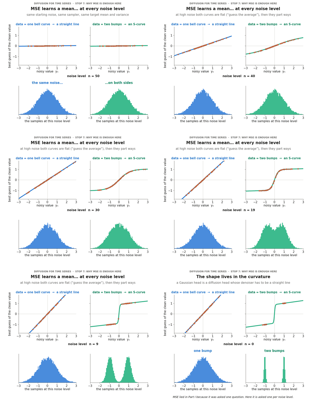
Animated comparability of two reverse diffusion processes that share the identical beginning noise, sampler and schedule. On the left the denoiser is the straight line that belongs to Gaussian information and produces one bump. On the appropriate it’s the S-curve that belongs to two-bump information and produces two bumps. It reveals {that a} Gaussian head is a diffusion head whose denoiser is restricted to a straight line.

Each runs goal at distributions with the identical imply and (as much as a small error that comes from utilizing solely fifty steps) the identical variance. The one distinction is whether or not the denoiser is a straight line or a curve, and that distinction alone decides whether or not we find yourself with one bump or with two. This offers us a exact method of stating the connection between the 2 sorts of head:

• A Gaussian head is a diffusion head whose denoiser is restricted to be a straight line. All the pieces a diffusion head can do past a Gaussian head lives within the curvature of what it learns.

• MSE lied in Half I as a result of it was requested a single query. In a diffusion mannequin it’s requested one query for each noise degree, and collectively the solutions describe the entire distribution.

7.4 Do extra steps make the mannequin extra correct?

Partly, and it’s value separating two sources of error. The primary is the dimension of the steps: every reverse step is modelled as one bell curve, which is actual just for infinitely small steps, so this error shrinks when $N$ grows, even with an ideal community. The second is the community itself, which has to be taught the conditional imply precisely at each noise degree; extra steps don’t enhance this, and small errors of the community accumulate alongside the chain. The primary error may be measured in isolation with the no-network setup of the earlier part, the place the denoiser is actual.

···

8. Producing a forecast worth: working the movie backwards

As soon as the community is educated, drawing one pattern works as follows. We begin from pure noise, $y_N sim mathcal{N}(0, 1)$

First, we ask the community for the noise it believes is contained within the present worth, $hatvarepsilon = varepsilon_theta(y_n, n)$

$mu = a_n,underbrace{y_n}_{textual content{the place we are actually}} ;+; c_n,underbrace{hat{y}_0}_{textual content{finest guess of the place we got here from}}$

Third, we compute the centre of the reverse step with the method of the cheat sheet, utilizing our guess $hat{y}_0$

$y_{n-1} = underbrace{textcolor{#2B6CB0}{mu}}_{textual content{centre from the community}} ;+; underbrace{textcolor{#2F9E5B}{tildesigma_n, z}}_{textual content{just a little contemporary noise}}, qquad z sim mathcal{N}(0, 1)$

And fourth, we take the step by including just a little contemporary noise, $y_{n-1} = mu + tildesigma_n, z$

Discover that the fourth operation is precisely the road mu + sigma * randn with which the Gaussian head of Half I attracts a pattern.

Earlier than attaching this to a forecaster, the pocket book trains the smallest doable diffusion mannequin, one which generates a single quantity with no context in any respect, on the two-bump information of Part 1. It takes just a few seconds, and it’s a good second to persuade your self that the equipment of the final 4 sections works earlier than the rest is added.

···

9. The experiment: a sign that basically branches

9.1 The information

We’d like a sign on which the issue of Part 1 truly happens, and ideally one for which we all know the true reply, so that each mannequin may be checked in opposition to it. I’ll use the ball from Part 1, now as a correct simulation that produces a time sequence.

The ball rolls in a panorama with two wells, one at $x = -1$

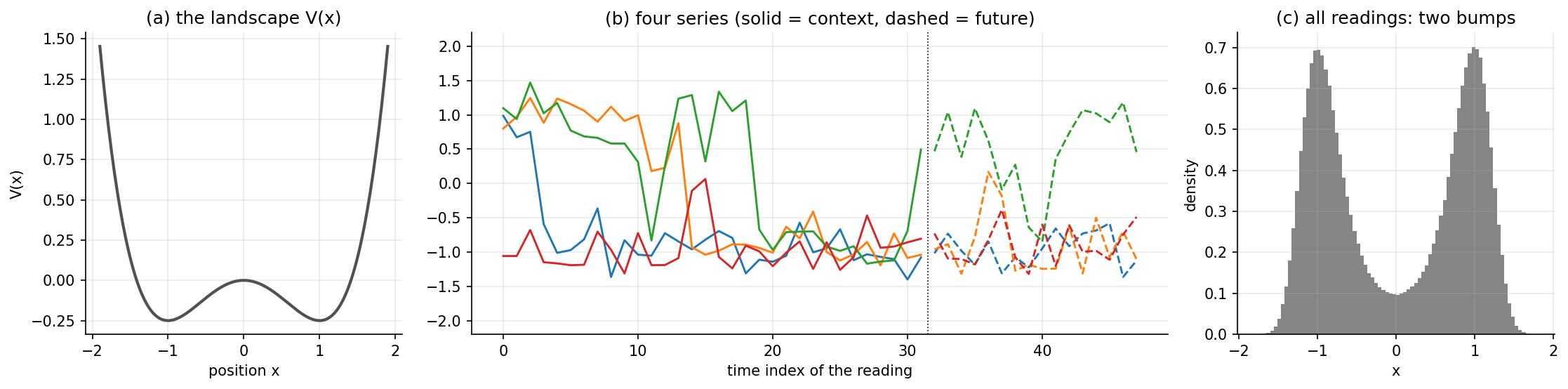
This dataset is an effective take a look at for 2 causes. The longer term can actually department, as a result of a ball that sits close to the barrier can fall into both nicely. And we all know the true reply, as a result of the physics has no reminiscence past the present place, so for any context we will restart the simulator from the final studying as typically as we like. That is the “repeat the identical state of affairs a thousand instances” (Part 1.1) made actual, and it provides us samples of the true distribution of futures. As within the earlier elements, the mannequin sees a context of $T = 32$

9.2 Plugging the diffusion head into the forecaster

The step that connects every little thing again to the earlier articles is a small one. The forecaster of Elements I and II had an encoder that reads the context and compresses it right into a abstract vector $mathbf{h}$, and two heads that flip $mathbf{h}$ right into a imply and a variance. We preserve the encoder and change the heads:

context x_1 ... x_T --> ENCODER --> h --> HEAD --> a pattern of the subsequent worth Gaussian head (Elements I and II): mu(h), sigma(h) one draw: mu + sigma * noise Diffusion head (this half) : eps(y_n, n, h) N = 50 small attracts in a row

···

10. Outcomes

We practice two forecasters on the double nicely which might be an identical in each respect apart from the top, in order that any distinction between them is a distinction within the form they’re allowed to specific. For every of the 1,000 take a look at contexts we then roll out $M = 100$

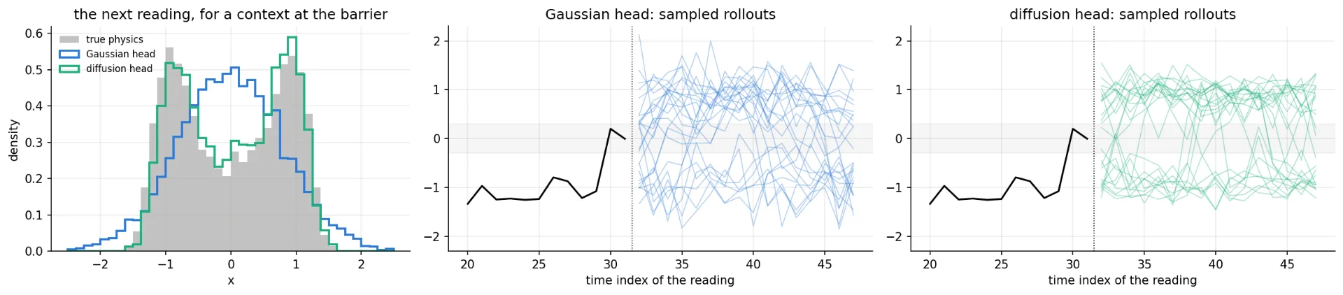
Forecasts for a context that ends on the barrier. Left: the true distribution of the subsequent studying has two bumps with a dip between them; the Gaussian head provides one broad bump centred on the dip, and the diffusion head reproduces each bumps. Center and proper: 25 sampled rollouts from the Gaussian head and from the diffusion head, with the barrier area shaded.

Most of the Gaussian paths begin within the barrier area, hesitate there for just a few steps and solely then drift to 1 facet, whereas the diffusion paths depart the barrier shortly and decide to a nicely, as the true ball does.

To place numbers on this over all take a look at contexts, I exploit the Steady Ranked Chance Rating (CRPS), which for forecast samples $X$ and $X’$ and an noticed worth $y$ is:

$mathrm{CRPS} = mathbb{E},lvert X – y rvert – tfrac{1}{2},mathbb{E},lvert X – X’ rvert$

The primary time period rewards samples that land near what truly occurred, and the second provides credit score again for trustworthy unfold, so {that a} mannequin shouldn’t be punished for being unsure when the long run actually is unsure. Decrease is healthier, and since a part of the long run is genuinely random, even the true physics doesn’t rating zero.

By the CRPS, the 2 heads are virtually tied: $0.494$ in opposition to $0.493$. But Determine 10 reveals a distinction that no one might miss, and the second column places a quantity on it, the barrier share, which is the fraction of forecast values that fall into the area $lvert x rvert < 0.3$

There’s a lesson right here that goes past diffusion fashions. A single abstract quantity hides a distinction in threat in Half I, and right here a much more subtle abstract quantity hides a distinction in form, so each time you may, have a look at the samples.

···

11. Prices and limits

None of that is free, and it could not be within the spirit of this sequence to faux in any other case. The prices:

• Sampling time. One trajectory of sixteen steps prices$16 instances 50 = 800$

• No method. With two heads you may learn off $mu$ and $sigma$ and compute any chance in closed kind. With a diffusion head, each interval or threshold chance must be estimated from samples, which is fortuitously what Half II taught us to do anyway.

• Coaching time. Roughly 5 instances longer for the diffusion head, nicely over a minute in opposition to lower than twenty seconds.

• A small bias from few steps. As Part 7 defined, with$N = 50$

And the bounds of the experiment:

• Simple information. The information is one-dimensional and artificial, and the system has no reminiscence past its final studying, which makes the job of the encoder simple which explains why we all know the true reply. For a similar motive the pocket book makes use of a small multilayer perceptron because the encoder as an alternative of the transformer of Elements I and II; the transformer may be swapped again in with out touching the heads.

• One run, no tuning. The outcomes come from one random seed and from small networks with none tuning.

• Comparisons I not noted. I didn’t practice a mix density community, which might deal with this specific downside nicely so long as someone tells it that there are two bumps, and I didn’t forecast the entire horizon in a single shot, since each would have distracted from the one comparability this text is about.

The place to learn extra

This text took one path by means of diffusion fashions, the one which results in forecasting the subsequent worth of a sign. The introductions beneath take different paths, almost all of them by means of pictures, they usually complement this one nicely. I record them by what you could be in search of, with the sections of this text they correspond to.

If you would like footage and plain language first.

• Introduction to Diffusion Fashions for Machine Studying by Ryan O’Connor (AssemblyAI) explains the ahead and the reverse course of with clear diagrams and contrasts diffusion with earlier generative fashions.

• A Light Introduction to Diffusion by Brett Younger (Weights & Biases) is a visible stroll by means of noise schedules and noise prediction.

• Diffusion Fashions: A Sensible Information (Scale AI) is about utilizing picture mills in apply, and is the place to go in case your curiosity is in producing footage and never within the mechanism.

If you would like the total idea.

• What are Diffusion Fashions? by Lilian Weng is the usual reference. It derives the decrease sure of our Part 6 for vectors, in full generality, and goes on to subjects I not noted, equivalent to quicker samplers and steerage.

• Understanding Diffusion Fashions: A Unified Perspective by Calvin Luo builds as much as diffusion from variational autoencoders and reveals that predicting the clear worth, predicting the noise and predicting the “rating” are three views of the identical factor.

What none of them does, so far as I do know, is what this text is about: denoising a single future worth of a time sequence, given its previous, inside an autoregressive rollout, and checking the end result in opposition to a identified reality.

···

References

• J. Ho, A. Jain, P. Abbeel, Denoising Diffusion Probabilistic Fashions, NeurIPS 2020.

• A. Nichol, P. Dhariwal, Improved Denoising Diffusion Probabilistic Fashions, ICML 2021 (the cosine schedule).

• C. M. Bishop, Combination Density Networks, Technical Report, Aston College, 1994.

• D. P. Kingma, M. Welling, Auto-Encoding Variational Bayes, ICLR 2014 (steady hidden variables and the ELBO).

• Ok. Rasul, C. Seward, I. Schuster, R. Vollgraf, Autoregressive Denoising Diffusion Fashions for Multivariate Probabilistic Time Collection Forecasting (TimeGrad), ICML 2021.

• T. Li, Y. Tian, H. Li, M. Deng, Ok. He, Autoregressive Picture Era with out Vector Quantization (MAR), NeurIPS 2024.

• C. M. Bishop, H. Bishop, Deep Studying: Foundations and Ideas, Springer, 2024, Chapters 15, 16 and 20.

• T. Gneiting, A. E. Raftery, Strictly Correct Scoring Guidelines, Prediction, and Estimation, Journal of the American Statistical Affiliation, 2007 (CRPS).