“Los Movimientos”: The Routing Drawback That Practically Broke My Spirit

that will immediately fill you with dread.

Phrases that make your shoulders tense the second you hear them. Phrases that create that unusual void in your abdomen, like when an elevator drops somewhat too quick.

Obtained them?

For me, these phrases have been:

Los Movimientos — “The actions,” in English.

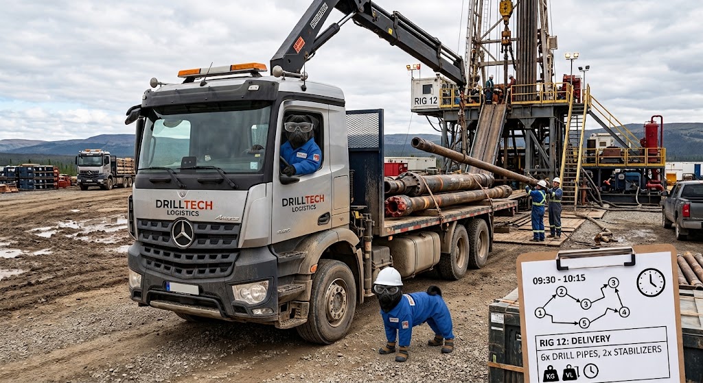
Again once I labored in oil and fuel, my colleagues Jesús B, Karina G. and I have been liable for planning and coordinating each motion of instruments and personnel required by the drilling operations throughout jap Venezuela for a serious oilfield companies firm.

And when exercise was at its peak, there have been numerous actions.

We have been supporting round 50 drilling jobs per 30 days. On any given day, roughly a dozen heavy vans may be dispatched to ship or acquire drilling instruments, whereas one other dozen gentle pickup vans transported directional-drilling crews between operational bases, resorts, and lively drilling rigs.

Most actions concerned delivering one thing from the operational base to a rig, or bringing instruments and personnel again from the sphere. However generally we additionally had lateral actions between rigs: acquire a device from Rig A, ship it to Rig B, decide up a crew some place else, and someway get everybody the place they wanted to be earlier than the driving restrictions kicked in.

Each afternoon, often round 4 p.m., the requests began arriving.

Not one after the other, calmly and politely.

They arrived as a flock.

Discipline service managers would ship the required device actions, personnel actions, pressing pickups, rig-to-rig transfers, and last-minute adjustments. From that pile of requests, I needed to assemble the route of each truck and each pickup for the next day.

And the automobiles didn’t essentially start on the operational base. Their beginning areas relied on the place they’d completed the day before today. A truck may be parked on the base, at a rig, or some place else totally. The identical was true for the crews.

To make issues extra entertaining, driving after 8 p.m. was forbidden besides underneath distinctive circumstances.

And no, this was not some annoying bureaucratic rule invented to make our lives harder. We have been continually reminded that street accidents have been among the many biggest risks in oilfield operations. Transferring individuals and heavy gear throughout lengthy distances, typically on poor roads and after exhausting shifts, was critical enterprise.

So each route needed to work.

The automobile wanted sufficient capability. It needed to start within the right location. It needed to acquire every merchandise earlier than delivering it. The crew wanted to be picked up earlier than they might be dropped off. The truck needed to attain every rig at an inexpensive time. And all the pieces needed to end earlier than the night driving restriction.

Let me let you know: this job was soul-crushing.

Planning every truck felt like fixing a horrible maze mixed with a tough Sudoku puzzle, besides the Sudoku puzzle might name you the following morning and let you know that you just had f*cked it up.

I might simply spend a number of hours each afternoon planning the routes. I did it with pen and paper.

Properly, pen, paper, and an Excel spreadsheet.

However Excel was not serving to a lot.

I’d finally end, take a look at the plan, and persuade myself that all the pieces made sense. Then, the next morning, I’d uncover that one route was infeasible, {that a} device couldn’t arrive on time, {that a} automobile had been assigned some place else, or {that a} sequence I had proposed merely didn’t work.

Then all the pieces needed to change once more.

It was deeply demoralizing.

Maybe you will have skilled one thing related. There’s a specific type of frustration that comes from not understanding how one can do your job properly and, even worse, having completely no concept how one can enhance.

You already know there should be a greater method. You think that somebody, someplace, has already solved an identical drawback. However you don’t even know what phrases to sort into Google.

That was precisely the place I used to be.

This was 2015–2016. There was no ChatGPT, no Claude, and no useful chatbot ready to elucidate vehicle-routing fashions to an exhausted drilling engineer at 5 within the afternoon.

I searched on-line for issues like “transportation planning,” “truck routing,” and “logistics optimization.”

What did I discover?

Largely commercials from trucking corporations and generic logistics blogs explaining that transportation was necessary.

Thanks. Very useful.

The one genuinely helpful factor Jesús and I discovered was an article saying that we would have liked to assemble a distance matrix. So we started doing precisely that.

Jesús, Karina, we have been heading in the right direction.

However, analytically talking, we have been additionally so extremely far-off.

It was like going to a physician understanding that you just have been sick, however not understanding what illness you had, what sort of specialist you wanted, and even how one can describe the signs.

The place do you start whenever you have no idea the identify of the issue?

The worst half was that, from the surface, none of this seemed notably tough.

Different individuals would casually assume that planning the actions needs to be straightforward. Simply assign a couple of vans, draw some routes, and ship them out.

However I’ve not but advised you essentially the most painful half.

We didn’t have a devoted fleet.

The heavy vans and pickups got here from a shared pool utilized by a number of oilfield service segments. My section was drilling, however different enterprise traces have been competing for a similar automobiles. If one truck was assigned to us, that was one truck unavailable to a different operation.

So we weren’t merely making an attempt to design good routes.

We have been making an attempt to design them with scarce assets, underneath time restrictions, with unsure beginning areas, paired pickup-and-delivery necessities, vehicle-capacity limits, and fixed competitors for the fleet.

It felt like combating a battle that had already been misplaced.

At this time, after finishing a PhD in economics and spending most of my analysis life working in operations analysis, I lastly know what sort of monster we have been combating.

And let me let you know, it was a tricky motherf*cker.

So, Jesús and Karina in case you are studying this: we had no probability.

We did the very best we might with the instruments and data we had. Actually, it’s type of miraculous that we managed to maintain the whole operation operating that method.

The monster even has a kind of absurdly lengthy names that sounds just like the title of a medieval king:

The Capacitated Pickup and Supply Automobile Routing Drawback with Time Home windows

How the f*ck have been we speculated to seek for that in 2015?

And even when, by means of some miracle, we had found the right identify, have you ever seen the mathematical formulation of this factor?

Don’t worry. You will note it within the subsequent sections.

But when I had encountered these equations again then, with out my present coaching, I’d have assumed they have been arcane magic. Unusual runes written by some secret society of mathematicians who had by no means skilled the enjoyment of receiving twelve pressing transportation requests at 4:45 p.m.

The formulation appears to be like terrible.

It appears to be like dense, intimidating, and virtually intentionally indigestible.

However the underlying logic will not be magic. It’s merely a exact method of describing the identical nightmare Jesús and I have been making an attempt to resolve each afternoon with paper, instinct, and a barely helpful Excel sheet.

That’s the reason I’m writing this text.

Maybe you might be at present in the identical place I used to be in. Maybe you might be planning deliveries, collections, service visits, technicians, medical transportation, warehouse transfers, or area crews. Maybe your present course of is inefficient, however you have no idea what the issue is known as or the place to start out.

I don’t need you to battle with it with out understanding what you might be coping with.

I see this text as a present to my earlier self: the reason and dealing instance I desperately wanted again then.

And if considered one of my former colleagues who remains to be working in oil and fuel occurs to learn this, particularly now that there’s renewed discuss of accelerating drilling exercise in Venezuela, please:

Strive planning Los Movimientos this manner.

It would assist. Loads.

On this article, we are going to:

• Translate the real-world nightmare of Los Movimientos into a proper pickup-and-delivery routing drawback.
• Perceive the principle components of the issue, together with automobiles, pickup areas, supply areas, capacities, journey instances, and time home windows.
• Construct a small however lifelike instance that captures the important difficulties of the unique operation.
• Formulate the issue as a mixed-integer linear programming mannequin.
• Clarify every resolution variable, constraint, and objective-function time period in plain language.
• Implement the whole mannequin in Python utilizing Pyomo.
• Remedy the mannequin with the open-source HiGHS optimizer.
• Extract the optimized automobile routes from the answer.
• Visualize the ensuing pickup-and-delivery plan.
• Talk about the restrictions of the mannequin and the way it might be prolonged to bigger and extra lifelike operations.

By the top, you should have an entire working instance that you could adapt to your personal transportation, field-service, or last-mile supply drawback.

The Drawback: When Each Supply Additionally Comes with a Pickup

At first look, a supply drawback sounds easy.

A buyer locations an order, a automobile leaves the depot, delivers the product, and strikes on to the following buyer.

However many actual transportation operations will not be that easy.

Typically, the automobile should not solely ship one thing, but in addition decide one thing up.

That is extraordinarily frequent in trendy retail, e-commerce, and last-mile logistics.

Think about grocery supply companies that use reusable containers. A driver might ship milk, juice, or different merchandise in returnable bottles or crates, whereas gathering the empty containers from a earlier order.

The identical logic seems in furnishings and household-appliance supply. An organization might ship a brand new fridge, washer, couch, or mattress whereas additionally gathering the client’s outdated one. In some nations, together with France, this sort of take-back service is frequent and should even be required in sure conditions.

The automobile due to this fact performs two related operations:

1. Decide up an merchandise at one location.
2. Ship that very same merchandise to a different location.

Typically the path is reversed from what we often think about. The automobile delivers a brand new product to the client after which collects an outdated product that should be transported again to a warehouse, recycling heart, or disposal facility.

These paired operations create what is called a pickup-and-delivery request.

The important thing phrase right here is paired.

If a automobile collects an merchandise, that very same merchandise should finally be delivered someplace. Extra importantly, the pickup should occur earlier than the supply.

You can’t ship a fridge that you haven’t but collected.

You can’t drop off a drilling device at a rig if the truck has not first picked it up from the operational base.

You can’t return an empty bottle to the distribution heart if the motive force has not but visited the client.

This creates a priority relationship between the 2 areas.

And that’s solely the start.

Time home windows make all the pieces tougher

Clients will not be at all times obtainable all through the whole day.

A family might request supply between 8 a.m. and midday. A retailer might solely settle for deliveries earlier than opening hours. A warehouse might cease receiving vans after 4 p.m. A drilling rig might require a device earlier than the beginning of a vital operation.

These restrictions are represented utilizing time home windows.

For every pickup or supply location, we outline an interval:

$$[a_i,b_i]$$the place:

• $a_i$ ​ is the earliest time service can start;
• $b_i$ is the newest time service can start.

A automobile might arrive early, but it surely should wait till the time window opens. If it arrives after the closing time, the go to is not possible.

Time home windows might come up for a number of causes.

Some are customer-related. A buyer might solely be obtainable throughout a particular interval.

Others come from operational restrictions. Warehouses, shops, development websites, hospitals, and industrial services might solely obtain automobiles throughout sure hours.

Cities may prohibit the circulation of heavy automobiles throughout components of the day. A truck could also be allowed to enter a neighborhood solely within the morning, or it might be forbidden from circulating throughout peak visitors hours.

Corporations may function underneath service-level agreements. A same-day order might should be delivered inside six hours. A medical pattern might have to succeed in a laboratory earlier than a deadline. A spare half might must arrive earlier than a upkeep crew can start its work.

Within the case of Los Movimientos, the time restriction was notably strict: automobiles have been typically not allowed to drive after 8 p.m or earlier than 6 a.m. Each route due to this fact needed to be accomplished inside that window.

Capability issues too

Autos can not carry a vast quantity of products.

A small pickup truck might transport a couple of containers or a crew of staff. A heavy truck might carry a number of massive drilling instruments, however even that truck has a most capability.

Which means that the order of the visits issues.

Suppose a automobile has capability for ten items. It can not decide up three orders of 5 items every earlier than delivering any of them. In some unspecified time in the future, it will be carrying fifteen items, which is unimaginable.

The route should due to this fact be designed in order that the automobile load by no means exceeds its capability.

Pickups improve the load of the automobile.

Deliveries lower it.

This creates one other dynamic component: the quantity carried by the automobile adjustments repeatedly alongside the route.

Not each automobile can serve each request

Actual fleets are hardly ever completely homogeneous.

Some requests require refrigerated automobiles. Others require vans with lifting gear, sufficient cargo house, particular permits, or drivers with specific {qualifications}.

In oilfield operations, sure instruments might solely be transported by specific sorts of vans. Personnel actions required gentle pickups, whereas heavy gear required bigger automobiles.

The mannequin should due to this fact account for compatibility.

A request could also be assigned solely to a automobile that’s bodily and operationally able to performing it.

Autos might begin elsewhere

Many textbook routing issues assume that each automobile begins and ends on the identical depot.

Actuality is usually messier.

A truck might start the day on the operational base. One other might have spent the night time at a drilling rig. A 3rd might begin at a upkeep facility after being repaired.

The identical automobile may end the day someplace completely different from the place it began.

This issues as a result of the beginning place of a automobile determines which requests it might probably serve effectively.

A truck already situated close to a pickup level could also be a more sensible choice than one which should journey two hours earlier than starting the route.

Typically there will not be sufficient automobiles

That is the place the issue turns into particularly painful.

The corporate might obtain extra transportation requests than the obtainable fleet can deal with.

Some requests might then need to be postponed, outsourced, or left unserved.

Within the formulation we are going to use, unserved requests are positioned in what the unique authors name a request financial institution. The optimization mannequin applies a big penalty to every request left there, encouraging the solver to function many requests as potential.

That is helpful as a result of it prevents the whole mannequin from turning into infeasible when the obtainable automobiles are inadequate.

As a substitute of merely declaring, “No resolution exists,” the mannequin tells us:

That is the very best plan potential with the automobiles at present obtainable, however these requests can’t be served.

That is a vital distinction in observe.

The Mannequin

So what precisely are we making an attempt to resolve? Given:

• a set of pickup-and-delivery requests;
• a fleet of automobiles;
• automobile capacities;
• journey instances and distances;
• time home windows;
• vehicle-request compatibility;
• beginning and ending areas;
• and presumably too few automobiles;

we should decide:

• which automobile serves every request;
• the order wherein every automobile visits its areas;
• when service begins at each location;
• how the automobile load adjustments alongside the route;
• and which requests, if any, should stay unserved.

The objective is to assemble routes which can be possible whereas minimizing a mixture of:

• complete distance travelled;
• complete working time;
• and the variety of unserved requests.

That is the Capacitated Pickup and Supply Drawback with Time Home windows.

And now that the monster has a reputation, we are able to lastly start describing it mathematically. We’re going to use the formulation described by Psinger et al. 2006 [1] that the authors describe because the PDPTW.

At first look, the formulation appears to be like intimidating, however the logic is definitely fairly pure. The mannequin is solely making an attempt to reply a sensible query:

Which automobile ought to do which pickup-and-delivery jobs, in what order, at what time, and with out violating capability or timing restrictions?

The mannequin does this by selecting automobile routes whereas minimizing complete transportation value.

The goal operate on the high minimizes three issues without delay:

1. Complete distance traveled by all automobiles.
2. Complete time spent by the automobiles on their routes.
3. The variety of requests left unserved.

That third time period is necessary. If there will not be sufficient automobiles or the requests are too tough to schedule, the mannequin is allowed to depart some requests out, but it surely pays a penalty for doing so. In observe, this penalty is often set excessive in order that the mannequin tries very arduous to serve all the pieces.

Earlier than wanting on the constraints, it helps to grasp the variables.

• x tells us whether or not a automobile goes straight from one location to a different.
  In plain English, this variable builds the precise route.
• S tells us the time at which a automobile begins service at a location.
  That is how the mannequin retains monitor of timing.
• L tells us the load of the automobile after servicing a location.
  That is how the mannequin retains monitor of capability.
• z tells us whether or not a request is left unserved.
  Whether it is, that request goes into the request financial institution.

Constraint (1): each request should be dealt with someway

Constraint (1) says that every request should have precisely one final result:

• both it’s assigned to a appropriate automobile,
• or it’s left unserved.

So the mannequin can not by chance overlook a request, and it can not assign the identical request to a number of automobiles.

Constraint (2): pickup and supply should be executed by the identical automobile

Constraint (2) ensures that if a automobile performs the pickup of a request, then that very same automobile should additionally carry out the corresponding supply.

That is important. In any other case, the mannequin might create nonsense options the place one truck picks up an merchandise and one other truck magically delivers it later.

So this constraint retains the pickup and supply linked collectively as one coherent job.

Constraint (3): each automobile should depart its place to begin

Constraint (3) says that every automobile should depart precisely as soon as from its begin terminal.

In sensible phrases, each automobile route should start someplace particular, corresponding to a depot, a base, or wherever that automobile is parked in the beginning of the day.

Constraint (4): each automobile should finish at its ending level

Constraint (4) says that every automobile should arrive precisely as soon as at its finish terminal.

So every route has a transparent finish in addition to a transparent starting.

Collectively, constraints (3) and (4) be sure that each automobile follows one full route from a begin location to an finish location.

Constraint (5): route continuity

Constraint (5) is the flow-conservation constraint.

It says that if a automobile arrives at a pickup or supply node, it should additionally depart that node.

This prevents unimaginable conditions the place a automobile:

• seems at a location with out getting there, or
• arrives at a location after which disappears.

That is what makes the chosen arcs kind a steady route fairly than a disconnected assortment of actions.

Constraint (6): time should transfer ahead alongside the route

Constraint (6) is without doubt one of the most necessary ones.

It says that if a automobile goes from location A to location B, then the beginning of service at B should occur after:

• service at A is accomplished, and
• the journey time from A to B has handed.

In on a regular basis phrases: a automobile can not teleport.

If it masses one thing at one place, spends a while there, after which drives to the following place, the clock should mirror that.

This constraint additionally helps eradicate bizarre round subroutes, as a result of time should preserve shifting ahead.

Constraint (7): each go to should respect its time window

Constraint (7) enforces the time home windows.

Every location has an earliest and newest allowable service time. This constraint ensures that the automobile begins service inside that interval.

This could symbolize many real-life restrictions, corresponding to:

• buyer availability,
• warehouse opening hours,
• supply deadlines,
• circulation restrictions in a metropolis,
• or, in my oil-and-gas story, the prohibition on driving too late within the day.

Constraint (8): pickup should occur earlier than supply

Constraint (8) enforces priority.

It says that the pickup of a request should occur earlier than the supply of that very same request.

This can be a easy concept, however a vital one.

A truck can not ship a device to a drilling website earlier than it has first collected it.
A supply crew can not eliminate an outdated washer earlier than it has first picked it up from the client.

This constraint enforces that logical order.

Constraint (9): the automobile load should evolve appropriately

Constraint (9) retains monitor of the automobile load from one cease to the following.

When a automobile visits a pickup location, its load will increase.

When it visits a supply location, its load decreases.

This constraint ensures that the load variable at all times matches what the automobile ought to truly be carrying alongside the route.

With out this, the mannequin might produce routes that ignore the bodily motion of the products.

Constraint (10): capability can’t be exceeded

Constraint (10) makes certain that the load of the automobile at all times stays between zero and its most capability.

Which means:

• the automobile can not carry greater than it’s bodily capable of transport,
• and it can not have a detrimental load.

So this prevents unimaginable plans corresponding to loading an excessive amount of gear onto one truck.

Constraint (11): automobiles begin and finish empty

Constraint (11) says that each automobile begins empty and should additionally end empty.

This is smart in pickup-and-delivery operations, as a result of something collected in the course of the route is meant to be delivered someplace earlier than the route ends.

So the mannequin doesn’t permit a automobile to complete the day with undelivered items nonetheless on board.

Constraint (12): routing selections are binary

Constraint (12) says that the routing variable can solely take the worth 0 or 1.

So for any potential motion, the reply is:

• sure, the automobile makes use of that arc,
• or no, it doesn’t.

There isn’t any midway worth.

Constraint (13): unserved-request selections are binary

Constraint (13) says that the request-bank variable can be binary.

So every request is both:

• unserved,
• or not unserved.

Once more, there is no such thing as a in-between.

Constraint (14): time and cargo can’t be detrimental

Constraint (14) says that the service instances and automobile masses should be nonnegative. That merely guidelines out meaningless values like detrimental time or detrimental cargo.

The Drawback Knowledge

Now that the mathematical monster has been launched, allow us to give it one thing sufficiently small to eat.

The actual model of Los Movimientos concerned dozens of automobiles, altering beginning areas, a number of enterprise items competing for a similar fleet, last-minute requests, and sufficient uncertainty to break anybody’s afternoon. Reproducing all of that right here can be lifelike, however it will additionally flip this tutorial into one other nightmare.

So we are going to work with a simplified day of personnel transportation.

Our small community accommodates one operational base and 5 drilling rigs. Three pickup vans can be found, and every one begins and ends the day on the operational base.

Firm coverage limits each pickup to 4 individuals, together with the motive force. Which means that every automobile can transport at most three passengers at any given time.

The working day begins at 6:00 a.m. and ends at 8:00 p.m. No automobile might depart earlier than 6:00 a.m., and each route should be accomplished by 8:00 p.m. As a result of the mannequin explicitly tracks journey and repair instances, it can not schedule a automobile to start a journey that will end after the cutoff.

We are going to take into account ten transportation requests, every composed of 1 pickup and one supply. This offers us twenty service nodes in complete.

The requests embody the three conditions we incessantly encountered within the area:

• personnel leaving the operational base to start work at a rig;
• personnel being transferred from one rig to a different;
• personnel ending their shift and returning to the operational base.

Each group should be collected earlier than it may be delivered, the identical pickup truck should carry out each components of the motion, and the truck must not ever carry greater than three passengers.

Every pickup and supply additionally has a time window. Some crews want to succeed in a rig earlier than the start of a shift, whereas others can solely be collected after finishing their work. We are going to assume that boarding or dropping off a bunch takes ten minutes.

To maintain the give attention to the routing mannequin, the three automobiles are an identical and may serve each request. Journey instances and distances are additionally assumed to be deterministic and symmetric. These assumptions will not be totally lifelike, however they offer us a clear occasion that HiGHS can remedy rapidly whereas preserving the important construction of the issue.

Request	Origin	Vacation spot	Passengers	Pickup window	Supply window
R01	Operational Base	Rig A	2	06:00–06:30	06:45–07:45
R02	Operational Base	Rig B	1	06:00–06:45	06:50–08:00
R03	Operational Base	Rig C	3	06:30–07:00	07:15–08:30
R04	Rig A	Rig D	2	08:00–08:30	08:50–10:00
R05	Rig B	Rig E	2	08:15–08:45	09:10–10:50
R06	Rig C	Rig A	2	08:30–09:00	09:15–11:00
R10	Rig B	Rig C	1	11:30–12:30	12:30–14:00
R07	Rig D	Operational Base	2	13:30–14:30	14:55–17:00
R08	Rig E	Operational Base	1	15:00–16:00	16:25–18:30
R09	Rig A	Operational Base	3	16:00–17:00	16:45–19:00

Though that is solely a toy occasion, it isn’t utterly trivial. A number of requests have overlapping time home windows, some teams occupy most of a automobile’s capability, and the automobiles should coordinate morning departures, rig-to-rig transfers, and night returns. The entire toy occasion, together with the automobile knowledge, location coordinates, travel-time matrix, distance matrix, service instances, and time home windows, is saved in a JSON file. The info for this drawback is obtainable in my Github-Repo.

So lets proceed to put in our solver and modelling framework, in addition to obtain the info, straight from the github repo.

!pip -q set up pyomo highspy

import json
from collections import defaultdict

import matplotlib.pyplot as plt
import numpy as np
import pandas as pd
import pyomo.environ as pyo
import requests

from IPython.show import show
from pyomo.choose import SolverFactory, TerminationCondition

JSON_URL = (
    "https://uncooked.githubusercontent.com/ceche1212/los_movimientos/"
    "refs/heads/principal/knowledge/los_movimientos_toy_instance.json"
)

response = requests.get(JSON_URL, timeout=30)
response.raise_for_status()
occasion = response.json()

print("Occasion loaded efficiently")
print(f"Title: {occasion['instance_name']}")
print(f"Autos: {len(occasion['vehicles'])}")
print(f"Requests: {len(occasion['requests'])}")
print(f"Service nodes: {2 * len(occasion['requests'])}")

The primary line installs Pyomo and the HiGHS solver. The remaining code imports the required libraries, downloads the JSON occasion straight from GitHub, converts it right into a Python dictionary, and shows its primary dimensions. Now that the JSON file has been loaded, we first create a small helper operate to transform instances expressed as minutes after midnight into a well-recognized clock format. We then use it to current the transportation requests as a readable desk.

def minutes_to_clock(minutes):
    """Convert minutes after midnight into HH:MM format."""
    minutes = int(spherical(minutes))
    return f"{minutes // 60:02d}:{minutes % 60:02d}"


request_rows = []

for request in occasion["requests"]:
    pickup = request["pickup"]
    supply = request["delivery"]

    request_rows.append({
        "request": request["id"],
        "motion sort": request["movement_type"],
        "origin": pickup["location"],
        "vacation spot": supply["location"],
        "passengers": request["passengers"],
        "pickup window": (
            f"{minutes_to_clock(pickup['time_window'][0])}–"
            f"{minutes_to_clock(pickup['time_window'][1])}"
        ),
        "supply window": (
            f"{minutes_to_clock(supply['time_window'][0])}–"
            f"{minutes_to_clock(supply['time_window'][1])}"
        )
    })

request_table = (
    pd.DataFrame(request_rows)
    .sort_values("pickup window")
    .reset_index(drop=True)
)

show(request_table)

Subsequent, we rework the nested JSON construction into the units and dictionaries that might be utilized by Pyomo. This consists of the automobiles, requests, pickup and supply nodes, time home windows, passenger adjustments, capacities, and automobile terminals.

automobiles = [v["id"] for v in occasion["vehicles"]]
request_ids = [r["id"] for r in occasion["requests"]]

vehicle_record = {v["id"]: v for v in occasion["vehicles"]}
request_record = {r["id"]: r for r in occasion["requests"]}

pickup_node = {
    r: request_record[r]["pickup"]["node_id"]
    for r in request_ids
}

delivery_node = {
    r: request_record[r]["delivery"]["node_id"]
    for r in request_ids
}

passengers = {
    r: request_record[r]["passengers"]
    for r in request_ids
}

compatible_vehicles = {
    r: request_record[r].get("compatible_vehicles", automobiles.copy())
    for r in request_ids
}


service_nodes = []
node_location = {}
earliest = {}
newest = {}
service_time = {}
load_change = {}
node_type = {}
node_request = {}

for request_id in request_ids:
    request = request_record[request_id]

    pickup = request["pickup"]
    pickup_id = pickup["node_id"]

    service_nodes.append(pickup_id)
    node_location[pickup_id] = pickup["location"]
    earliest[pickup_id], newest[pickup_id] = pickup["time_window"]
    service_time[pickup_id] = pickup["service_time"]
    load_change[pickup_id] = request["passengers"]
    node_type[pickup_id] = "pickup"
    node_request[pickup_id] = request_id

    supply = request["delivery"]
    delivery_id = supply["node_id"]

    service_nodes.append(delivery_id)
    node_location[delivery_id] = supply["location"]
    earliest[delivery_id], newest[delivery_id] = supply["time_window"]
    service_time[delivery_id] = supply["service_time"]
    load_change[delivery_id] = -request["passengers"]
    node_type[delivery_id] = "supply"
    node_request[delivery_id] = request_id


start_node = {okay: f"START_{okay}" for okay in automobiles}
end_node = {okay: f"END_{okay}" for okay in automobiles}

capability = {}
start_time = {}
end_time = {}
vehicle_nodes = {}

for vehicle_id in automobiles:
    automobile = vehicle_record[vehicle_id]

    capability[vehicle_id] = automobile["capacity_passengers"]
    start_time[vehicle_id] = automobile["start_time"]
    end_time[vehicle_id] = automobile["end_time"]

    begin = start_node[vehicle_id]
    finish = end_node[vehicle_id]

    node_location[start] = automobile["start_location"]
    earliest[start] = newest[start] = automobile["start_time"]
    service_time[start] = load_change[start] = 0
    node_type[start] = "begin"
    node_request[start] = None

    node_location[end] = automobile["end_location"]
    earliest[end] = automobile["start_time"]
    newest[end] = automobile["end_time"]
    service_time[end] = load_change[end] = 0
    node_type[end] = "finish"
    node_request[end] = None

    compatible_nodes = [
        node
        for request_id in request_ids
        if vehicle_id in compatible_vehicles[request_id]
        for node in (
            pickup_node[request_id],
            delivery_node[request_id]
        )
    ]

    vehicle_nodes[vehicle_id] = compatible_nodes + [start, end]


print(f"Autos: {len(automobiles)}")
print(f"Requests: {len(request_ids)}")
print(f"Service nodes: {len(service_nodes)}")

This preprocessing step converts the uncooked occasion right into a solver-friendly construction. Pickup nodes add passengers to a automobile, supply nodes take away them, and every truck receives its personal begin and finish terminal.

With the nodes and automobile knowledge ready, we are able to now assemble the potential actions between them. To maintain the optimization mannequin smaller, we instantly take away unimaginable arcs, corresponding to actions coming into a begin terminal, leaving an finish terminal, or reaching a vacation spot after its time window has already closed.

travel_matrix = occasion["travel_time_minutes"]
distance_matrix = occasion["distance_km"]

arcs, arc_travel_time, arc_distance = [], {}, {}

for okay in automobiles:
    begin, finish = start_node[k], end_node[k]

    for i in vehicle_nodes[k]:
        if i == finish:
            proceed

        for j in vehicle_nodes[k]:
            if j == begin or i == j:
                proceed

            origin, vacation spot = node_location[i], node_location[j]
            journey = travel_matrix[origin][destination]

            if earliest[i] + service_time[i] + journey > newest[j]:
                proceed

            arc = (okay, i, j)
            arcs.append(arc)
            arc_travel_time[arc] = journey
            arc_distance[arc] = distance_matrix[origin][destination]


outgoing, incoming = defaultdict(listing), defaultdict(listing)

for okay, i, j in arcs:
    outgoing[k, i].append(j)
    incoming[k, j].append(i)


vehicle_node_pairs = [
    (k, i)
    for k in vehicles
    for i in vehicle_nodes[k]
]

compatible_pairs = [
    (k, r)
    for r in request_ids
    for k in compatible_vehicles[r]
]

service_node_pairs = [
    (k, i)
    for k in vehicles
    for i in service_nodes
    if i in vehicle_nodes[k]
]

print(f"Variety of possible arcs: {len(arcs)}")

The ensuing arc set accommodates solely actions that would doubtlessly seem in a possible route. The incoming and outgoing dictionaries will later make the route-continuity constraints a lot simpler to assemble.

The time, priority, and passenger-load constraints should be relaxed at any time when their related motion or request will not be chosen, that is executed by way of one thing known as Huge-M constraint. Quite than utilizing one excessively massive quantity for M, we calculate smaller values tailor-made to every arc and request (this improves solver efficiency).

M_time = {
    (okay, i, j): max(
        0,
        newest[i]
        + service_time[i]
        + arc_travel_time[k, i, j]
        - earliest[j]
    )
    for okay, i, j in arcs
}

M_load = {
    (okay, i, j): capability[k] + max(0, load_change[j])
    for okay, i, j in arcs
}

M_precedence = {
    (okay, r): max(
        0,
        newest[pickup_node[r]]
        - earliest[delivery_node[r]]
    )
    for okay, r in compatible_pairs
}

These arc-specific values deactivate the corresponding constraints when crucial, whereas avoiding unnecessarily massive constants that would make the mannequin slower or numerically weaker.

Modelling the PDPTW

With the community and Huge-M values prepared, we are able to lastly translate the mathematical formulation into Pyomo.

mannequin = pyo.ConcreteModel(identify="Los_Movimientos_PDPTW")

# Units
mannequin.Okay = pyo.Set(initialize=automobiles)
mannequin.R = pyo.Set(initialize=request_ids)
mannequin.KV = pyo.Set(dimen=2, initialize=vehicle_node_pairs)
mannequin.KR = pyo.Set(dimen=2, initialize=compatible_pairs)
mannequin.KN = pyo.Set(dimen=2, initialize=service_node_pairs)
mannequin.A = pyo.Set(dimen=3, initialize=arcs)

# Variables
mannequin.x = pyo.Var(mannequin.A, area=pyo.Binary)
mannequin.z = pyo.Var(mannequin.R, area=pyo.Binary)
mannequin.S = pyo.Var(
    mannequin.KV,
    bounds=lambda m, okay, i: (earliest[i], newest[i])
)
mannequin.L = pyo.Var(
    mannequin.KV,
    bounds=lambda m, okay, i: (0, capability[k])
)

for okay in automobiles:
    mannequin.L[k, start_node[k]].repair(0)
    mannequin.L[k, end_node[k]].repair(0)

# Movement helpers
def outflow(m, okay, i):
    return sum(m.x[k, i, j] for j in outgoing[k, i])

def influx(m, okay, j):
    return sum(m.x[k, i, j] for i in incoming[k, j])

# (1) Each request is served or left unserved
mannequin.RequestAssignment = pyo.Constraint(
    mannequin.R,
    rule=lambda m, r:
        sum(outflow(m, okay, pickup_node[r])
            for okay in compatible_vehicles[r])
        + m.z[r] == 1
)

# (2) The identical automobile performs pickup and supply
mannequin.SameVehicle = pyo.Constraint(
    mannequin.KR,
    rule=lambda m, okay, r:
        outflow(m, okay, pickup_node[r])
        == influx(m, okay, delivery_node[r])
)

# (3)–(5) Begin, finish, and route continuity
mannequin.StartTerminal = pyo.Constraint(
    mannequin.Okay,
    rule=lambda m, okay: outflow(m, okay, start_node[k]) == 1
)

mannequin.EndTerminal = pyo.Constraint(
    mannequin.Okay,
    rule=lambda m, okay: influx(m, okay, end_node[k]) == 1
)

mannequin.FlowConservation = pyo.Constraint(
    mannequin.KN,
    rule=lambda m, okay, i: influx(m, okay, i) == outflow(m, okay, i)
)

# (6) Time propagation
def time_rule(m, okay, i, j):
    return (
        m.S[k, i] + service_time[i] + arc_travel_time[k, i, j]
        <= m.S[k, j] + M_time[k, i, j] * (1 - m.x[k, i, j])
    )

mannequin.TimePropagation = pyo.Constraint(mannequin.A, rule=time_rule)

# (8) Pickup earlier than supply
def precedence_rule(m, okay, r):
    pickup, supply = pickup_node[r], delivery_node[r]
    return (
        m.S[k, pickup]
        <= m.S[k, delivery]
        + M_precedence[k, r] * (1 - outflow(m, okay, pickup))
    )

mannequin.PickupBeforeDelivery = pyo.Constraint(
    mannequin.KR,
    rule=precedence_rule
)

# (9) Passenger-load propagation
def load_rule(m, okay, i, j):
    return (
        m.L[k, i] + load_change[j]
        <= m.L[k, j] + M_load[k, i, j] * (1 - m.x[k, i, j])
    )

mannequin.LoadPropagation = pyo.Constraint(mannequin.A, rule=load_rule)

# Goal elements
mannequin.TotalDistance = pyo.Expression(
    expr=sum(
        arc_distance[k, i, j] * mannequin.x[k, i, j]
        for okay, i, j in mannequin.A
    )
)

mannequin.TotalDuration = pyo.Expression(
    expr=sum(
        mannequin.S[k, end_node[k]] - start_time[k]
        for okay in mannequin.Okay
    )
)

mannequin.UnservedCount = pyo.Expression(
    expr=sum(mannequin.z[r] for r in mannequin.R)
)

mannequin.TotalCost = pyo.Goal(
    expr=(
        mannequin.TotalDistance
        + 0.05 * mannequin.TotalDuration
        + 10_000 * mannequin.UnservedCount
    ),
    sense=pyo.reduce
)

The code creates the routing, service-time, passenger-load, and unserved-request variables earlier than implementing the project, route-continuity, timing, priority, and capability logic. The target then minimizes complete distance, automobile working time, and a big penalty for any request that can’t be served.

Now that the Pyomo mannequin is full, we move it to the open-source HiGHS solver. We request an actual optimum resolution, impose a two-minute time restrict, and confirm that the solver terminates efficiently.

solver = SolverFactory("appsi_highs")

solver.highs_options.replace({
    "output_flag": True,
    "log_to_console": True,
    "mip_rel_gap": 0.0,
    "time_limit": 120
})

outcomes = solver.remedy(mannequin, tee=True)
termination = outcomes.solver.termination_condition

print("nTermination situation:", termination)

if termination != TerminationCondition.optimum:
    increase RuntimeError(
        f"HiGHS didn't discover an optimum resolution: {termination}"
    )

The solver log reveals how HiGHS processes the mixed-integer mannequin. The ultimate examine stops the pocket book if an optimum resolution will not be discovered, stopping us from deciphering an incomplete or infeasible consequence. After few seconds, that is the result of the solver.

Extracting the answer

HiGHS returns the chosen arcs fairly than a ready-made itinerary. We due to this fact join these arcs into an ordered route for every truck and print the consequence within the format an operator might truly use.

# Get better the chosen successor of each visited node
successor = {
    (okay, i): j
    for okay, i, j in mannequin.A
    if pyo.worth(mannequin.x[k, i, j]) > 0.5
}

# Reconstruct every route from its begin to its finish terminal
routes = {}

for okay in automobiles:
    route = [start_node[k]]

    whereas route[-1] != end_node[k]:
        present = route[-1]

        if (okay, present) not in successor:
            increase RuntimeError(f"Incomplete route for {okay} at {present}.")

        next_node = successor[k, current]

        if next_node in route and next_node != end_node[k]:
            increase RuntimeError(f"Cycle detected within the route of {okay}.")

        route.append(next_node)

    routes[k] = route


# Print an operator-friendly itinerary
for okay, route in routes.objects():
    distance = sum(
        arc_distance[k, i, j]
        for i, j in zip(route[:-1], route[1:])
    )

    print(f"n{'=' * 72}")
    print(f"{okay} | Complete distance: {distance:.1f} km")
    print(f"{'=' * 72}")

    onboard = 0

    for cease, node in enumerate(route):
        onboard += load_change[node]

        request = (
            f" | Request {node_request[node]}"
            if node_request[node]
            else ""
        )

        print(
            f"{cease:>2}. "
            f"{minutes_to_clock(pyo.worth(mannequin.S[k, node]))}"
            f" | {node_location[node]:<18}"
            f" | {node_type[node].title():<8}"
            f"{request:<16}"
            f" | Passengers onboard: {onboard}"
        )

The routes dictionary shops the ordered sequence wanted for the plots. The printed output then provides operators the deliberate time, location, exercise, related request, and variety of passengers onboard after each cease. The passenger depend is calculated straight from the sequence of pickups and deliveries, making certain that the displayed load displays the precise itinerary. Right here under are the ultimate routes produced by the solver.

======================================================================
Route for PU_1
======================================================================
06:00 | BASE               | begin    | Passengers onboard: 0
06:00 | BASE               | pickup   | Request: R01 | Passengers onboard: 2
06:45 | RIG_A              | supply | Request: R01 | Passengers onboard: 0
08:30 | RIG_A              | pickup   | Request: R04 | Passengers onboard: 2
10:00 | RIG_D              | supply | Request: R04 | Passengers onboard: 0
13:30 | RIG_D              | pickup   | Request: R07 | Passengers onboard: 2
14:55 | BASE               | supply | Request: R07 | Passengers onboard: 0
15:05 | BASE               | finish      | Passengers onboard: 0

======================================================================
Route for PU_2
======================================================================
06:00 | BASE               | begin    | Passengers onboard: 0
06:30 | BASE               | pickup   | Request: R03 | Passengers onboard: 3
07:25 | RIG_C              | supply | Request: R03 | Passengers onboard: 0
08:30 | RIG_C              | pickup   | Request: R06 | Passengers onboard: 2
09:15 | RIG_A              | supply | Request: R06 | Passengers onboard: 0
11:30 | RIG_B              | pickup   | Request: R10 | Passengers onboard: 1
12:30 | RIG_C              | supply | Request: R10 | Passengers onboard: 0
16:00 | RIG_A              | pickup   | Request: R09 | Passengers onboard: 3
16:45 | BASE               | supply | Request: R09 | Passengers onboard: 0
16:55 | BASE               | finish      | Passengers onboard: 0

======================================================================
Route for PU_3
======================================================================
06:00 | BASE               | begin    | Passengers onboard: 0
06:00 | BASE               | pickup   | Request: R02 | Passengers onboard: 1
08:00 | RIG_B              | supply | Request: R02 | Passengers onboard: 0
08:15 | RIG_B              | pickup   | Request: R05 | Passengers onboard: 2
09:20 | RIG_E              | supply | Request: R05 | Passengers onboard: 0
15:00 | RIG_E              | pickup   | Request: R08 | Passengers onboard: 1
16:25 | BASE               | supply | Request: R08 | Passengers onboard: 0
16:35 | BASE               | finish      | Passengers onboard: 0

At this level, we have already got the optimized itineraries for the three pickup vans. The ultimate step is to visualise them. To make the routes simpler to match, we plot every truck by itself panel whereas retaining the identical coordinate scale throughout the three subplots.

coordinates = occasion["locations"]
vehicle_ids = listing(routes.keys())

if len(vehicle_ids) != 3:
    increase ValueError(
        f"This visualization expects precisely three automobiles, however {len(vehicle_ids)} have been discovered."
    )

all_x = [loc["x_km"] for loc in coordinates.values()]
all_y = [loc["y_km"] for loc in coordinates.values()]
x_margin, y_margin = 5, 5

fig, axes = plt.subplots(1, 3, figsize=(20, 7), sharex=True, sharey=True)

for ax, okay in zip(axes, vehicle_ids):
    route = routes[k]

    for loc in coordinates.values():
        ax.scatter(loc["x_km"], loc["y_km"], s=100, zorder=3)
        ax.textual content(loc["x_km"] + 0.8, loc["y_km"] + 0.8, loc["name"], fontsize=9)

    x_values = [coordinates[node_location[node]]["x_km"] for node in route]
    y_values = [coordinates[node_location[node]]["y_km"] for node in route]

    ax.plot(x_values, y_values, marker="o", linewidth=2, zorder=2)

    for x0, y0, x1, y1 in zip(x_values[:-1], y_values[:-1], x_values[1:], y_values[1:]):
        if (x0, y0) != (x1, y1):
            ax.annotate(
                "",
                xy=(x1, y1),
                xytext=(x0, y0),
                arrowprops={"arrowstyle": "->", "alpha": 0.5, "linewidth": 1.5}
            )

    for s, node in enumerate(route):
        x = coordinates[node_location[node]]["x_km"]
        y = coordinates[node_location[node]]["y_km"]
        ax.annotate(
            str(s),
            xy=(x, y),
            xytext=(-8, -12),
            textcoords="offset factors",
            fontsize=8,
            fontweight="daring"
        )

    route_distance = sum(
        arc_distance[k, i, j]
        for i, j in zip(route[:-1], route[1:])
    )

    finish_time = pyo.worth(mannequin.S[k, end_node[k]])

    ax.set_title(f"{okay}n{route_distance:.1f} km | End: {minutes_to_clock(finish_time)}")
    ax.set_xlabel("x coordinate (km)")
    ax.grid(True, alpha=0.3)
    ax.set_xlim(min(all_x) - x_margin, max(all_x) + x_margin)
    ax.set_ylim(min(all_y) - y_margin, max(all_y) + y_margin)
    ax.set_aspect("equal", adjustable="field")

axes[0].set_ylabel("y coordinate (km)")
plt.tight_layout()
plt.present()

This determine provides one map per automobile. The arrows present the journey path, the small numbers point out the order of the stops, and the title of every subplot experiences the overall route distance and ending time.

Conclusions

And there we now have it: an entire optimization mannequin for Los Movimientos.

The mannequin provides us the optimum routes for the three pickup vans, at the very least with respect to the assumptions, knowledge, and goal operate used on this tutorial. However it does one thing much more beneficial: it tells us whether or not the present fleet is ample.

Bear in mind the penalty related to unserved requests. If the mannequin can not transport everybody whereas respecting the time home windows, automobile capacities, and pickup-before-delivery necessities, it doesn’t merely collapse and declare the whole drawback infeasible. As a substitute, it identifies the requests that can’t be served. Operationally, that offers us a really clear warning:

We might have one other truck.

Trying on the resolution, it’s tough to not admire the facility of optimization. HiGHS solved in a couple of seconds a puzzle that will as soon as have taken me a number of hours to deal with manually. Even after spending all that point, I couldn’t have assured that my routes have been optimum, and even that they have been utterly possible.

Route 2 is a very good instance. The truck makes what initially seems to be an pointless back-and-forth motion between a few of the rigs. A human planner would possibly instantly reject that route. Visiting the identical location greater than as soon as doesn’t look environment friendly.

To be trustworthy, I most likely would by no means have thought of it.

But the mannequin doesn’t care whether or not a route appears to be like elegant. It cares whether or not the route serves the requests, respects the time home windows, retains the passenger load inside capability, and minimizes the target. What appears to be like unusual to the human eye can nonetheless be completely possible and optimum.

That is without doubt one of the most fascinating issues about optimization: generally the very best resolution will not be the one our instinct would naturally produce.

A mannequin will not be but a usable system

There may be one other lesson right here that’s straightforward to miss.

In an actual operation, we couldn’t ask dispatchers to open a JSON file and manually encode each request. Pondering again to my crew of dispatchers, Wilfredo, Duirbel, and Gustavo, asking them to enter all the necessities straight into JSON would have been a horrible punishment.

Severely, what the f*ck would that workflow seem like?

A sensible implementation would require a easy graphical interface the place dispatchers might enter the origin, vacation spot, variety of passengers, pickup window, and supply deadline with out seeing any code in any respect. The applying would quietly convert their inputs into JSON, run the optimization mannequin, and return the really helpful routes.

This will likely sound secondary in contrast with the arithmetic, however it isn’t.

Optimization methods additionally fail due to poor person expertise. A mathematically sensible resolution is ineffective if the individuals liable for working it discover it uncomfortable, complicated, or unnecessarily difficult.

By no means disregard the human and behavioral facet of an optimization drawback. If the system is disagreeable to make use of, individuals will merely cease utilizing it, and even worst by no means use it.

Actual operations would require extra constraints

I intentionally stored this tutorial so simple as potential, and it nonetheless grew to become a behemoth of an article. However what did you anticipate? This can be a tough drawback.

An actual implementation would most likely require a number of extra operational guidelines.

For instance, we had a fatigue-management rule stating that if a driver operated repeatedly for greater than two hours, they wanted to take a 15-minute break earlier than persevering with. Nevertheless, if the motive force stopped at a rig throughout that interval, the cease already interrupted the continuous-driving time, and the extra break was pointless.

Representing this rule would require the mannequin to trace not solely complete route period, but in addition the quantity of uninterrupted driving because the earlier qualifying cease. That’s completely potential, however it will introduce extra variables and constraints.

Different functions may also require driver shifts, vehicle-specific {qualifications}, lunch breaks, emergency-priority requests, unsure journey instances, a number of depots, or requests arriving dynamically in the course of the day.

The mannequin offered right here is due to this fact not the ultimate phrase. It’s a basis.

When the precise mannequin turns into too massive

For this toy occasion, and almost definitely for the size of the operation I labored with in Venezuela, a mixed-integer linear mannequin solved with HiGHS would most likely have been completely sufficient.

HiGHS is a really succesful open-source solver, and the truth that we are able to remedy an issue like this with out buying a industrial license is genuinely spectacular.

Nevertheless, the scenario adjustments when the issue turns into a lot bigger.

Think about an e-commerce firm planning routes for a whole lot of pickup and supply areas throughout a big fleet. The variety of potential automobile actions grows extraordinarily rapidly, and an actual MILP (Blended Integer Linear Program) formulation might require a prohibitive period of time to show optimality.

At that scale, one choice is to make use of a strong industrial solver corresponding to Gurobi or CPLEX. They’re glorious, though their full industrial licenses will be costly.

Another choice is to cease demanding a mathematically confirmed optimum and as an alternative seek for a superb resolution inside an inexpensive period of time. That is exactly the strategy taken by Ropke and Pisinger, who proposed an Adaptive Giant Neighborhood Search heuristic for the pickup-and-delivery drawback with time home windows [1].

And that’s precisely the place we are going to go subsequent.

In Los Movimientos, Half II, we are going to depart the comfy world of tangible optimization and discover how Adaptive Giant Neighborhood Search can deal with a lot bigger variations of the issue.

I sincerely hope you discovered this text helpful and entertaining. I’d love to listen to your ideas, notably you probably have confronted a equally chaotic transportation, routing, or dispatching drawback. Be happy to depart a remark or present your appreciation with a clap 👏.

You can too comply with the newest work from Sávila Schooling and join with me on LinkedIn.

Thanks for taking the time to learn. And Jesús, Wilfredo, Duirbel, and Gustavo: we lastly solved Los Movimientos.

All the code and knowledge associated to this text will be discovered within the following Github-Repo.

References

[1] Ropke, S., & Pisinger, D. (2006). An adaptive massive neighborhood search heuristic for the pickup and supply drawback with time home windows. Transportation Science, 40(4), 455–472.