PANet Paper Walkthrough: When Characteristic Pyramids Go Backside-Up

LLM Wikis Are Over-Engineered — I Changed Mine With a Pure Python Compiler

Cease Returning Textual content from RAG: The Typed Reply Contract That Prevents Hallucination

I wrote concerning the FPN (Characteristic Pyramid Community) structure [1], which is likely one of the most influential necks we are able to apply to a spine mannequin. FPN was first launched to boost the aptitude of an object detection mannequin to detect small objects. Nonetheless, Liu et al. in 2018 discovered that the data move of FPN had room for enchancment. So, they determined to handle this hole by proposing PANet of their analysis paper titled “Path Aggregation Community for Occasion Segmentation” [2], which we’re going to talk about on this article.

A Little Bit About FPN

PANet is constructed on high of the FPN structure, so I feel it might be a good suggestion to speak just a little bit about how FPN works upfront. In a CNN-based spine mannequin, the deeper characteristic maps have completely different traits from the shallower ones. The characteristic maps from deeper layers are likely to have excessive semantic data, but it doesn’t have that a lot quantity of spatial data. Conversely, characteristic maps from shallower layers comprise extra spatial data however have much less semantic data. These info primarily inform us that we must always use the deeper characteristic maps if we had been to foretell massive objects and use the shallower characteristic maps for predicting small objects.

Nonetheless, the authors of PANet discovered that it isn’t fairly acceptable to straight take data from shallower characteristic maps to detect small objects. It is because these characteristic maps comprise minimal quantity of semantic data, which primarily implies that they don’t have an excellent understanding concerning the content material of the picture. FPN solves this challenge by combining characteristic maps from the deeper layers and the shallower ones. By doing so, we are able to principally inject semantic data into the shallower characteristic maps that they beforehand didn’t have.

What FPN Solves

Now check out the illustration in Determine 1 beneath to higher perceive this concept. The upward move on the left is the principle spine mannequin, whereas the one going downwards on the correct (a.okay.a. the top-down pathway) is the FPN. The horizontal arrows that go on to the FPN half (known as lateral connections) are the tensors to be mixed with the one from the deeper layers. On this illustration, the FPN produces three characteristic maps the place the detection head will make the bounding field predictions from.

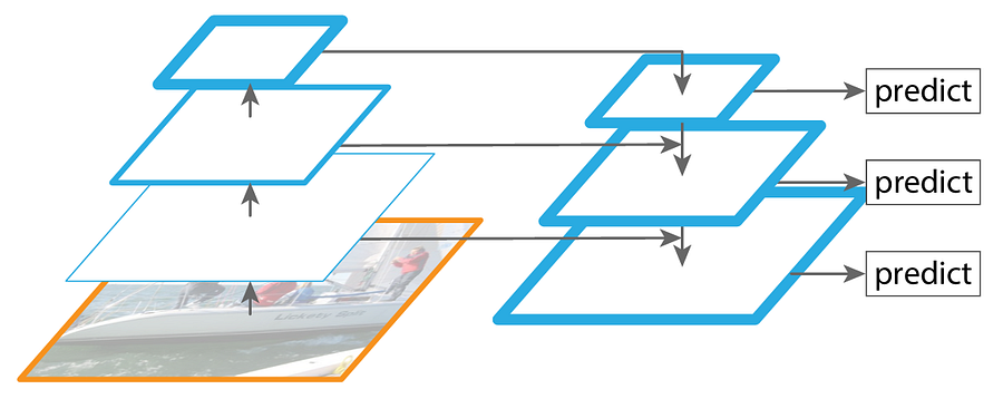
The blue borderlines within the illustration above point out the quantity of semantic data contained throughout the corresponding characteristic map. You may see within the unique spine that the borderline will get thicker as we get deeper into the community, that means that the characteristic map that has the best semantic data is the one produced by the deepest layer. Through the use of characteristic map mixture mechanism proposed by FPN, we are able to see that the shallower characteristic maps are actually wealthy of semantic data which makes them appropriate for detecting small objects precisely.

What FPN Doesn’t Resolve

At this level we would assume that FPN is simply positive because it is ready to permit a mannequin to detect small objects higher in comparison with the plain spine mannequin. Actually, the authors of PANet nonetheless see one thing that isn’t solved by FPN simply but, which as I’ve talked about earlier is expounded to the data move downside. Now let’s check out Determine 2 beneath.

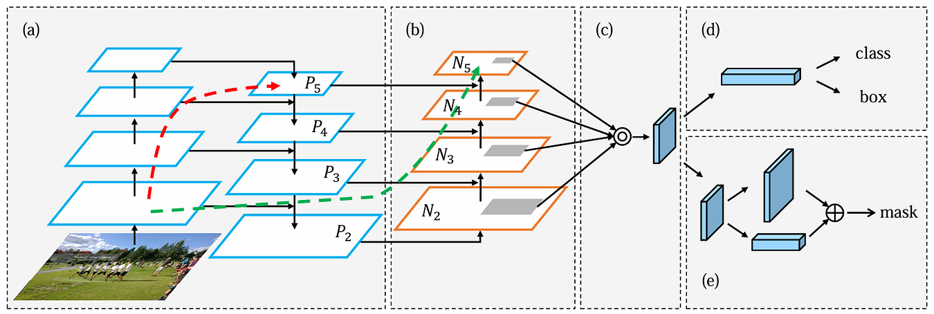
On this determine, the part known as (a) is the spine mannequin that has been outfitted with FPN, which is principally the identical construction I confirmed you in Determine 1. In FPN, characteristic maps P₅, P₄, P₃, and P₂ turn into the idea of the detection head to make predictions, the place P₂ has a excessive semantic data because of the move within the top-down pathway. And right here’s the issue FPN doesn’t resolve: whereas FPN successfully enriches characteristic maps in shallower layers, the deeper characteristic maps nonetheless lack spatial data. At first of this text I stated that the deeper and the shallower characteristic maps in a spine have their very own benefit and disadvantage, and FPN solely solves the downside of the shallower characteristic maps whereas nonetheless leaving the issue of the deeper characteristic maps untouched. Based mostly on this notion, the authors of PANet thought that we may nonetheless enhance the power of an object detection mannequin in detecting massive objects by injecting spatial data to the deeper characteristic maps, which additionally probably permits the general accuracy of the detection mannequin to get even greater.

It’s positively regular for a deeper layer to lose spatial data as a result of downsampling mechanism within the spine. Nonetheless, that is really not solely brought on by the downsampling itself. As an alternative, the lengthy data journey within the stack of convolution layers additionally causes spatial data to degrade. So, if we can’t omit the downsampling operation throughout the spine, we are able to nonetheless decrease this spatial data degradation by creating shortcut paths — identical to the skip-connections in ResNet.

How PANet Solves the Drawback Unsolved by FPN

The authors of PANet proposed a intelligent thought, the place they added a stack of a number of convolution layers positioned on high of the present FPN alongside the lateral connections (the half known as (b) in Determine 2). It might sound counterintuitive at look — how can including extra layers permit us to get shorter paths as an alternative? Actually, this method is legitimate because it actually permits the shallower characteristic maps to ship spatial data to the deeper layers extra seamlessly.

Now let’s return to Determine 2 and take note of the dashed arrows. Each arrows primarily denote the move of the C₂ tensor (the spine characteristic on the identical spatial decision as P₂ and N₂) to the deepest layer. The purple one is after we solely use the top-down pathway of FPN, whereas the inexperienced one is after we additionally use the bottom-up path augmentation of PANet.

If we don’t make the most of PANet, the one means for the C₂ tensor to get into the final layer P₅ is by touring up via all the spine one after the other, which may really be over 100 layers in complete. And as we mentioned earlier, this causes degradation within the spatial data. If we evaluate this with the move after we use PANet, it primarily permits us to make use of the trail traced by the inexperienced arrow. Needless to say the variety of layers throughout the top-down and the bottom-up pathways are a lot lower than the one within the spine, therefore decreasing the trail from 100+ layers to round 10 layers to succeed in N₅ (which is in the identical stage as P₅). By doing this, we are able to positively protect way more spatial data. And so, by combining FPN and PANet, we get bidirectional data move that enriches shallower layers with semantic data and deeper layers with spatial data.

By the best way, on this article we’ll concentrate on how we are able to combine the (a) and (b) elements within the structure, which is the core contribution that has been broadly adopted in trendy architectures. The total PANet paper really additionally consists of the adaptive pooling mechanism (c), bounding field prediction for object detection (d), and fully-connected characteristic fusion for segmentation (e), that are past our scope right here.

The Detailed PANet Structure

In FPN, the P₅, P₄, P₃, and P₂ tensors will straight be forwarded to the detection head, whereas in PANet, these 4 tensors can be transferred to the bottom-up path augmentation which then produces the N₅, N₄, N₃, and N₂ tensors. These N tensors are those for use by the detection head as the idea of the thing detection prediction.

Usually talking, the best way PANet performs characteristic mixture is just like FPN but is finished in reversed means. Check out Determine 3 beneath to see the detailed course of.

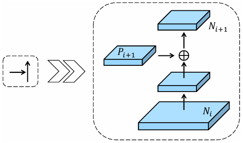
Determine 3. An illustration of the constructing block for bottom-up path augmentation [2].

What we initially do within the above constructing block is to course of the Nᵢ tensor with a 3×3 convolution. The stride of this conv layer is about to 2 since we wish it to scale back the spatial dimension by half. Subsequent, we mix the Pᵢ₊₁ tensor and the downsampled Nᵢ tensor utilizing element-wise summation. This mixed tensor is then processed by one other 3×3 convolution layer. This time we don’t need this layer to scale back the spatial dimension any additional, so we have to set the stride to 1. Lastly, as all processes above are completed, we may have the Nᵢ₊₁ tensor, which is able to be processed once more with the identical process till we finally get all of the N₅, N₄, N₃, and N₂ tensors.

There are literally a number of stuff you want to remember right here. First, since N₂ is the very first tensor within the bottom-up path augmentation, there may be really nothing to mix to acquire this tensor. Thus, we are able to merely understand P₂ because the N₂ tensor itself. Second, right here we have to put a ReLU activation perform after every convolution layer. Actually, that is completely different from FPN which fully omits the activation capabilities. So, later within the implementation, our top-down pathway is not going to use any activation perform in any respect, but we may have all of the convs within the bottom-up path augmentation outfitted with ReLU. And third, all tensors all through all the bottom-up path augmentation have precisely 256 channels, that means that the convolution layers right here don’t change the variety of channels in any respect.

That’s just about all concerning the detailed move of the PANet structure. Within the subsequent part I’m going to show learn how to implement it from scratch.

PANet From Scratch

The concept of our implementation right here is that we are going to create a dummy spine with an FPN and place the PANet layers on high of it. As typical, what we have to do first within the code is to import the required modules. See Codeblock 1 beneath.

# Codeblock 1
import torch
import torch.nn as nn

CNN Implementation

What I really imply by a dummy spine is a quite simple CNN mannequin. Actually the CNN class in Codeblock 2 beneath is strictly the identical because the one in my FPN article [1]. Simply remember the fact that the precise spine used within the paper is ResNet, however for the reason that focus of this text is PANet, I’ll use a normal CNN as an alternative. (By the best way, I really bought a separate article about ResNet. Test that out on the hyperlink in reference [4] in case you’re to implement FPN on ResNet from scratch.)

# Codeblock 2
class CNN(nn.Module):
    def __init__(self):
        tremendous().__init__()
        
        self.relu = nn.ReLU()
        self.maxpool = nn.MaxPool2d(kernel_size=3, stride=2, padding=1)
        
        self.conv1 = nn.Conv2d(in_channels=3, out_channels=64, kernel_size=3, padding=1)
        self.conv2 = nn.Conv2d(in_channels=64, out_channels=256, kernel_size=3, padding=1)
        self.conv3 = nn.Conv2d(in_channels=256, out_channels=512, kernel_size=3, padding=1)
        self.conv4 = nn.Conv2d(in_channels=512, out_channels=1024, kernel_size=3, padding=1)
        self.conv5 = nn.Conv2d(in_channels=1024, out_channels=2048, kernel_size=3, padding=1)
        
    def ahead(self, x):
        print(f'originalt: {x.measurement()}n')
        
        x = self.relu(self.conv1(x))
        print(f'after conv1t: {x.measurement()}')
        
        x = self.maxpool(x)
        print(f'after poolt: {x.measurement()}n')
        
        x = self.relu(self.conv2(x))
        print(f'after conv2t: {x.measurement()}')
        
        x = self.maxpool(x)
        print(f'after pool (c2)t: {x.measurement()}n')
        
        c2 = x.clone()
        
        x = self.relu(self.conv3(x))
        print(f'after conv3t: {x.measurement()}')
        
        x = self.maxpool(x)
        print(f'after pool (c3)t: {x.measurement()}n')
        
        c3 = x.clone()
        
        x = self.relu(self.conv4(x))
        print(f'after conv4t: {x.measurement()}')
        
        x = self.maxpool(x)
        print(f'after pool (c4)t: {x.measurement()}n')
        
        c4 = x.clone()
        
        x = self.relu(self.conv5(x))
        print(f'after conv5t: {x.measurement()}')
        
        c5 = self.maxpool(x)
        print(f'after pool (c5)t: {c5.measurement()}n')
        
        return c2, c3, c4, c5

The CNN class above returns a number of outputs: c2, c3, c4 and c5, the place c5 is the tensor from the deepest layer. To be able to verify if this class works correctly, we’ll check it by passing a tensor via it. The dummy tensor I initialize in Codeblock 3 beneath has the dimension of three×224×224, which matches the enter form of the ResNet mannequin.

# Codeblock 3
cnn = CNN()

x = torch.randn(1, 3, 224, 224)
out_cnn = cnn(x)

c2, c3, c4, c5 = out_cnn

Beneath you may see how the spine mannequin transforms our enter tensor all through the community. In a while, all of the C tensors can be used because the enter of our FPN.

# Codeblock 3 Output
unique        : torch.Measurement([1, 3, 224, 224])

after conv1     : torch.Measurement([1, 64, 224, 224])
after pool      : torch.Measurement([1, 64, 112, 112])

after conv2     : torch.Measurement([1, 256, 112, 112])
after pool (c2) : torch.Measurement([1, 256, 56, 56])

after conv3     : torch.Measurement([1, 512, 56, 56])
after pool (c3) : torch.Measurement([1, 512, 28, 28])

after conv4     : torch.Measurement([1, 1024, 28, 28])
after pool (c4) : torch.Measurement([1, 1024, 14, 14])

after conv5     : torch.Measurement([1, 2048, 14, 14])
after pool (c5) : torch.Measurement([1, 2048, 7, 7])

FPN Implementation

And right here’s what the FPN class appears like. I’m not going to get very deep into the move of this community since I’ve lined it totally in my earlier article [1].

# Codeblock 4
class FPN(nn.Module):
    def __init__(self):
        tremendous().__init__()
        
        self.upsample = nn.Upsample(scale_factor=2, mode='nearest')    #(1)
        
        self.lateral_c5 = nn.Conv2d(in_channels=2048, out_channels=256, kernel_size=1)
        self.lateral_c4 = nn.Conv2d(in_channels=1024, out_channels=256, kernel_size=1)
        self.lateral_c3 = nn.Conv2d(in_channels=512,  out_channels=256, kernel_size=1)
        self.lateral_c2 = nn.Conv2d(in_channels=256,  out_channels=256, kernel_size=1)
        
        self.smooth_m4  = nn.Conv2d(in_channels=256, out_channels=256, kernel_size=3, padding=1)
        self.smooth_m3  = nn.Conv2d(in_channels=256, out_channels=256, kernel_size=3, padding=1)
        self.smooth_m2  = nn.Conv2d(in_channels=256, out_channels=256, kernel_size=3, padding=1)
        
    def ahead(self, c2, c3, c4, c5):
        m5 = self.lateral_c5(c5)
        p5 = m5
        
        m4 = self.upsample(m5) + self.lateral_c4(c4)
        p4 = self.smooth_m4(m4)
        
        m3 = self.upsample(m4) + self.lateral_c3(c3)
        p3 = self.smooth_m3(m3)
        
        m2 = self.upsample(m3) + self.lateral_c2(c2)
        p2 = self.smooth_m2(m2)
        
        return p2, p3, p4, p5

For now, let’s simply concentrate on the returned P tensors which we’ll use because the enter of our PANet. You may see within the output of the code beneath that every one these P tensors have 256 channels, which I consider is why the authors finally ended up with this variety of channels for all the PANet construction.

# Codeblock 5
fpn = FPN()

out_fpn = fpn(c2, c3, c4, c5)
p2, p3, p4, p5 = out_fpn

print(f'p2: {p2.measurement()}')
print(f'p3: {p3.measurement()}')
print(f'p4: {p4.measurement()}')
print(f'p5: {p5.measurement()}')

# Codeblock 5 Output
p2: torch.Measurement([1, 256, 56, 56])
p3: torch.Measurement([1, 256, 28, 28])
p4: torch.Measurement([1, 256, 14, 14])
p5: torch.Measurement([1, 256, 7, 7])

PANet Implementation

And eventually, it’s time to implement the PANet itself. In Codeblock 6 beneath, what we do first is to initialize the downsample_n{2,3,4} layers. Because the identify suggests, these layers are liable for performing spatial downsampling, which is the rationale that we set the stride parameter of those layers to 2. Subsequent, we initialize conv_{n2down_p3, n3down_p4, n4down_p5}. These three convolution layers are used to course of the mixed tensors. As an example, the layer with suffix n2down_p3 will take the mixed downsampled N₂ and the P₃ tensors for the enter. Don’t overlook to initialize the ReLU activation perform as we’ll use them after every convolution layer.

# Codeblock 6
class PANet(nn.Module):
    def __init__(self):
        tremendous().__init__()
        
        self.downsample_n2 = nn.Conv2d(in_channels=256, out_channels=256, kernel_size=3, stride=2, padding=1)
        self.downsample_n3 = nn.Conv2d(in_channels=256, out_channels=256, kernel_size=3, stride=2, padding=1)
        self.downsample_n4 = nn.Conv2d(in_channels=256, out_channels=256, kernel_size=3, stride=2, padding=1)
        
        self.conv_n2down_p3 = nn.Conv2d(in_channels=256, out_channels=256, kernel_size=3, padding=1)
        self.conv_n3down_p4 = nn.Conv2d(in_channels=256, out_channels=256, kernel_size=3, padding=1)
        self.conv_n4down_p5 = nn.Conv2d(in_channels=256, out_channels=256, kernel_size=3, padding=1)
        
        self.relu = nn.ReLU()

    def ahead(self, p2, p3, p4, p5):
        
        n2 = p2                                         #(1)
        print(f'n2tt: {n2.measurement()}n')
        
        #######################################
        
        n2down = self.relu(self.downsample_n2(n2))      #(2)
        print(f'n2 downsampledt: {n2down.measurement()}')

        n2down_p3 = n2down + p3                         #(3)
        print(f'after sumt: {n2down_p3.measurement()}')
        
        n3 = self.relu(self.conv_n2down_p3(n2down_p3))  #(4)
        print(f'n3tt: {n3.measurement()}n')
        
        #######################################
        
        n3down = self.relu(self.downsample_n3(n3))
        print(f'n3 downsampledt: {n3down.measurement()}')
        
        n3down_p4 = n3down + p4
        print(f'after sumt: {n3down_p4.measurement()}')
        
        n4 = self.relu(self.conv_n3down_p4(n3down_p4))
        print(f'n4tt: {n4.measurement()}n')
        
        #######################################
        
        n4down = self.relu(self.downsample_n4(n4))
        print(f'n4 downsampledt: {n4down.measurement()}')
        
        n4down_p5 = n4down + p5
        print(f'after sumt: {n4down_p5.measurement()}')
        
        n5 = self.relu(self.conv_n4down_p5(n4down_p5))
        print(f'n5tt: {n5.measurement()}')
        
        return n2, n3, n4, n5

Now let’s transfer on to the ahead() methodology. You may see right here that we settle for all P tensors from FPN because the enter. As I’ve talked about earlier, we don’t have to do something with the P₂ tensor since its corresponding N tensor is the very first one within the bottom-up path augmentation (#(1)). Subsequent, on the line marked with #(2) we downsample the n2 tensor such that its spatial dimension halves. This downsampling course of is vital since we wish the n2 tensor to have the very same dimension as p3 to permit element-wise summation to be carried out (#(3)). Afterwards, this mixed tensor is processed additional by one other convolution layer (#(4)). These steps are repeated a number of occasions till we finally attain n5.

Now let’s check our code above by initializing a PANet occasion and move the P tensors we obtained from our earlier output via the community.

# Codeblock 7
panet = PANet()

out_panet = panet(p2, p3, p4, p5)
n2, n3, n4, n5 = out_panet

And beneath is what the output appears like. It looks as if our PANet works correctly because it efficiently passes the enter tensor all the best way to the top of the community. It’s also seen right here that whereas the spatial dimension will get smaller, the variety of characteristic maps in every step stays the identical, which is strictly what we wish.

# Codeblock 7 Output
n2             : torch.Measurement([1, 256, 56, 56])

n2 downsampled : torch.Measurement([1, 256, 28, 28])
after sum      : torch.Measurement([1, 256, 28, 28])
n3             : torch.Measurement([1, 256, 28, 28])

n3 downsampled : torch.Measurement([1, 256, 14, 14])
after sum      : torch.Measurement([1, 256, 14, 14])
n4             : torch.Measurement([1, 256, 14, 14])

n4 downsampled : torch.Measurement([1, 256, 7, 7])
after sum      : torch.Measurement([1, 256, 7, 7])
n5             : torch.Measurement([1, 256, 7, 7])

All the things in a Single Move

Lastly, let’s attempt to wrap the whole lot in a single class which I discuss with as BackboneNeck. The best way to do this can be very easy, all we have to do within the __init__() methodology is simply to initialize the dummy CNN, FPN, and the PANet we created earlier. Subsequent, within the ahead() methodology, we are able to simply move the tensors sequentially. Right here I additionally print out the form of the tensors within the intermediate steps with the intention to clearly see how the tensors remodel after every a part of the community. The outputs of this BackboneNeck are the N tensros, that are able to be forwarded to a detection head.

# Codeblock 8
class BackboneNeck(nn.Module):
    def __init__(self):
        tremendous().__init__()
        
        self.cnn   = CNN()
        self.fpn   = FPN()
        self.panet = PANet()
    
    def ahead(self, x):
        c2, c3, c4, c5 = self.cnn(x)
        print(f'c2: {c2.measurement()}')
        print(f'c3: {c3.measurement()}')
        print(f'c4: {c4.measurement()}')
        print(f'c5: {c5.measurement()}n')
        
        p2, p3, p4, p5 = self.fpn(c2, c3, c4, c5)
        print(f'p2: {p2.measurement()}')
        print(f'p3: {p3.measurement()}')
        print(f'p4: {p4.measurement()}')
        print(f'p5: {p5.measurement()}n')
        
        n2, n3, n4, n5 = self.panet(p2, p3, p4, p5)
        print(f'n2: {n2.measurement()}')
        print(f'n3: {n3.measurement()}')
        print(f'n4: {n4.measurement()}')
        print(f'n5: {n5.measurement()}')
        
        return n2, n3, n4, n5

Now let’s check our BackboneNeck class above utilizing the next testing code.

# Codeblock 9
backbone_neck = BackboneNeck()

x = torch.randn(1, 3, 224, 224)
n2, n3, n4, n5 = backbone_neck(x)

Right here we are able to see that our dummy RGB picture of measurement 224×224 efficiently flows via all the community. The C tensors produced by the spine initially have various numbers of channels (#(1–4)). Our FPN then normalizes them to a uniform 256 channels whereas enriching the shallower layers with semantic data (#(5–8)). We additional course of the ensuing P tensors with PANet to inject spatial data to the deeper layers, ensuing within the N tensors whereas sustaining the identical spatial dimensions as their corresponding P tensors (#(9–12)).

# Codeblock 9 Output
unique        : torch.Measurement([1, 3, 224, 224])

after conv1     : torch.Measurement([1, 64, 224, 224])
after pool      : torch.Measurement([1, 64, 112, 112])

after conv2     : torch.Measurement([1, 256, 112, 112])
after pool (c2) : torch.Measurement([1, 256, 56, 56])

after conv3     : torch.Measurement([1, 512, 56, 56])
after pool (c3) : torch.Measurement([1, 512, 28, 28])

after conv4     : torch.Measurement([1, 1024, 28, 28])
after pool (c4) : torch.Measurement([1, 1024, 14, 14])

after conv5     : torch.Measurement([1, 2048, 14, 14])
after pool (c5) : torch.Measurement([1, 2048, 7, 7])

c2: torch.Measurement([1, 256, 56, 56])    #(1)
c3: torch.Measurement([1, 512, 28, 28])    #(2)
c4: torch.Measurement([1, 1024, 14, 14])   #(3)
c5: torch.Measurement([1, 2048, 7, 7])     #(4)

p2: torch.Measurement([1, 256, 56, 56])    #(5)
p3: torch.Measurement([1, 256, 28, 28])    #(6)
p4: torch.Measurement([1, 256, 14, 14])    #(7)
p5: torch.Measurement([1, 256, 7, 7])      #(8)

n2: torch.Measurement([1, 256, 56, 56])    #(9)
n3: torch.Measurement([1, 256, 28, 28])    #(10)
n4: torch.Measurement([1, 256, 14, 14])    #(11)
n5: torch.Measurement([1, 256, 7, 7])      #(12)

Ending

And that’s the whole lot about how PANet works, particularly relating to the best way it enriches spatial data within the deeper layers. There are literally a number of different extra elements of PANet I haven’t lined on this article, i.e., the (c), (d), and (e) elements in Determine 2, which I feel I’ll reserve it for my upcoming articles.

Thanks very a lot for studying. You may as well discover the code used on this article in my GitHub repo [5]. Please let me know if there are errors within the code or in my rationalization. See ya in my subsequent article!

References

[1] Muhammad Ardi. FPN Paper Walkthrough: Leveraging the Inner Pyramid. https://towardsdatascience.com/fpn-paper-walkthrough-leveraging-the-internal-pyramid/ [Accessed July 3, 2026].
[2] Shu Liu et al. Path Aggregation Community for Occasion Segmentation. Arxiv. https://arxiv.org/abs/1803.01534 [Accessed October 8, 2025].
[3] Tsung-Yi Lin et al. Characteristic Pyramid Networks for Object Detection. Arxiv. https://arxiv.org/abs/1612.03144 [Accessed October 8, 2025].
[4] Muhammad Ardi. Paper Walkthrough: Residual Community (ResNet). Python in Plain English. https://medium.com/python-in-plain-english/paper-walkthrough-residual-network-resnet-62af58d1c521 [Accessed October 8, 2025].
[5] MuhammadArdiPutra. PANet. GitHub. https://github.com/MuhammadArdiPutra/medium_articles/blob/predominant/Deeppercent20Learningpercent20Frompercent20Scratch/PANet.ipynb [Accessed October 8, 2025].