


In my earlier submit, I 4 core improvements that makes ORPilot a production-oriented open-source LLM-for-OR instrument, particularly interview agent, information assortment agent, parameter computation agent and intermediate illustration (IR). Among the many 4 improvements, the IR is an important one which differentiates ORPilot from an instructional prototype and endows it with the potential to be a production-level instrument, because it offers with two points {that a} manufacturing atmosphere cares most about: reproducibility and portability. On this submit, I offers you a deep dive into ORPilot’s IR construction.
What Is IR?
There’s a drawback that nearly no one talks about when discussing AI-generated optimization fashions: what occurs after the primary clear up?
You get your mannequin working. You get an optimum answer. After which three weeks later, you want to re-run it with up to date demand information. Or your colleague on a special machine wants to breed the outcome. Or your organization decides to change from Gurobi to an open-source solver due to licensing prices. Otherwise you wish to ask “what if we enhance the capability of a facility by 20%?” With most present LLM-for-OR instruments, the reply to all of those questions is similar: you want to begin over, name the LLM once more, pay the API price once more, generate the solver code once more, and hope to get the identical mannequin construction. Nonetheless, the open-source AI optimization modeling agent ORPilot offers an alternate answer to this drawback: Intermediate Illustration (IR).
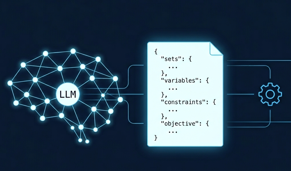
The IR is a solver-agnostic, typed JSON schema that captures the entire mathematical construction of an optimization mannequin. Not the optimization code, however the mannequin itself, expressed in a kind that’s impartial of any explicit solver.
ORPilot’s IR construction has 5 top-level sections.
(1) Units: named collections of entities, akin to Employees, Duties, Vegetation, Durations. Every set is aware of the place its members come from: a CSV file, a scalar depend, or a hardcoded record.
(2) Parameters: listed numerical information from CSV recordsdata, every linked to its area (which units index it) and to the precise column names wanted to load it.
(3) Variables: resolution variables with kind (steady, binary, integer), area, bounds, and structural flags.
(4) Goal: a symbolic expression tree over variables and parameters — sums, variations, merchandise, listed sums in solver-neutral kind.
(5) Constraints: named symbolic constraints with domains, expression bushes, and sense (<= or = or >=). Each constraint is an entire, self-describing object.
Let’s make this concrete by taking a look at a selected employee job task drawback beneath.
Employee-Process Task Downside Instance
On this drawback, 4 staff have to be assigned to 4 duties, one job per employee, one employee per job. Every (employee, job) pair has a price from a CSV file. We attempt to reduce the overall task price. This can be a basic task drawback, which is an integer program.
The info lives in two recordsdata:
(1) units.csv (all set members in a single place):
set_name factor
staff w1
staff w2
staff w3
staff w4
duties t1
duties t2
duties t3
duties t4
(2) assignment_costs.csv (the price matrix):
worker_id task_id price
w1 t1 2.0
w1 t2 4.0
… … …
Right here is the complete IR for this drawback:
{
    "problem_class": "AssignmentProblem",
    "model_type": "Combined Integer Program",
    "sense": "reduce",

    "units": {
      "Employees": {
        "dimension": null,
        "index_symbol": "w",
        "supply": "units.csv",
        "column": "factor",
        "filter_column": "set_name",
        "filter_value": "staff",
        "ordered": false
      },
      "Duties": {
        "dimension": null,
        "index_symbol": "t",
        "supply": "units.csv",
        "column": "factor",
        "filter_column": "set_name",
        "filter_value": "duties",
        "ordered": false
      }
    },

    "parameters": {
      "assignment_cost": {
        "area": ["Workers", "Tasks"],
        "kind": "float",
        "supply": "assignment_costs.csv",
        "column": "price",
        "index_columns": ["worker_id", "task_id"],
        "missing_default": "inf"
      }
    },

    "variables": {
      "assign": {
        "description": "1 if employee w is assigned to job t, 0 in any other case",
        "label": "assignments",
        "area": ["Workers", "Tasks"],
        "kind": "binary",
        "lower_bound": 0,
        "upper_bound": 1,
        "upper_bound_set": null,
        "exclude_diagonal": false,
        "domain_filter": null
      }
    },

    "constraints": {
      "one_task_per_worker": {
        "area": ["Workers"],
        "expression": {
          "operation": "indexed_sum",
          "over": ["Tasks:t"],
          "physique": {"kind": "variable", "title": "assign", "indices": ["w", "t"]}
        },
        "sense": "=",
        "rhs": {"kind": "fixed", "worth": 1}
      },
      "one_worker_per_task": {
        "area": ["Tasks"],
        "expression": {
          "operation": "indexed_sum",
          "over": ["Workers:w"],
          "physique": {"kind": "variable", "title": "assign", "indices": ["w", "t"]}
        },
        "sense": "=",
        "rhs": {"kind": "fixed", "worth": 1}
      }
    },

    "goal": {
      "sense": "reduce",
      "expression": {
        "operation": "indexed_sum",
        "over": ["Workers:w", "Tasks:t"],
        "physique": {
          "operation": "multiply",
          "left":  {"kind": "parameter", "title": "assignment_cost", "indices": ["w", "t"]},
          "proper": {"kind": "variable",  "title": "assign",          "indices": ["w", "t"]}
        }
      }
    }
  }
Let’s stroll by way of what every part is doing and why the design choices had been made.
Units
The “units” discipline signifies the place set members come from. An important design resolution in “units” is the info supply conference. ORPilot requires all set members to stay in a single file known as units.csv, utilizing a two-column format: “set_name” and “factor”. Each set — entities (staff, duties, crops) and time units (durations, months) is a filtered slice of this file. On this drawback, the “Employees” discipline says: load members from units.csv, learn the “factor” column, preserve solely rows the place “set_name” column equals “staff”. The outcome at compile time shall be Employees = [“w1”, “w2”, “w3”, “w4”].
This conference has two advantages. First, all grasp information is in a single place. Including a employee means including a row to units.csv, not modifying a number of recordsdata. Second, the “filter_value” discipline is verified towards the precise distinct values in units.csv at IR-generation time, catching typos earlier than the solver code produces empty units. The “index_symbol” discipline (“w” for Employees, “t” for Duties) is the loop variable title that may seem within the complied solver code, e.g., “for w in Employees, for t in Duties”. It have to be chosen to keep away from image conflicts throughout nested loops (see the shadow rule beneath). The “ordered” discipline is fake for each units right here, but it surely turns into crucial for time-indexed fashions. An ordered set helps temporal lag references, e.g., referencing stock[t-1] from inside a period-t constraint.
Parameters
The “parameters” discipline hyperlinks information to the mannequin. The “assignment_cost” parameter has six structural fields.
(1) “area”: [“Workers”, “Tasks”] — this parameter is listed by each units, producing a 2D desk.
(2) “kind”: “float” — the info kind of this parameter is float.
(3) “supply”: “assignment_costs.csv” — the precise filename (with extension) that holds the info.
(4) “column”: “price” — the CSV column that holds the numeric values to load.
(5) “index_columns”: [“worker_id”, “task_id”] — the CSV columns that function keys, in the identical order as “area”. The “index_columns” discipline is among the most consequential items of the IR. With out it, the compiler can not decide which columns within the CSV correspond to which area units. Traditionally, a typical failure mode was the compiler guessing the incorrect key column title and silently loading the incorrect information. The IR enforces that the right column names are all the time provided explicitly.
(6) “missing_default”: “inf” — tells the compiler that any (employee, job) pair not current within the CSV must be handled as having infinite price, which means that route is unavailable. That is the right semantic for price and penalty parameters.
Variables
The “variables” discipline defines the choices to be made within the optimization mannequin. The “assign” variable is binary, listed over “area”: [“Workers”, “Tasks”]. In order that at compile time, the compiler builds (assuming utilizing PuLP solver):
assign = {(w, t): pulp.LpVariable(f"assign_{w}_{t}", cat="Binary") for w in Employees for t in Duties}Some key structural flags not used right here however price understanding are “exclude_diagonal”, “domain_filter” and “upper_bound_set”.
For variables listed over the identical set twice, like “arc[Location, Location]” in a routing mannequin, setting “exclude_diagonal=true” tells the compiler to skip the (i, i) diagonal. No location travels to itself. The compiler emits an
if l1 == l2:
   proceed
guard and makes use of “.get(key, 0)” for all accesses so lacking keys by no means trigger “KeyError”.
When a price desk has fewer rows than the complete Cartesian product of its area units (e.g. solely legitimate routes exist within the CSV), setting “domain_filter” to that parameter’s title restricts the variable to solely these combos. The compiler emits the comprehension with “if (i, j) in transport_cost” so non-existent routes are by no means created as variables.
For integer variables whose pure higher certain is the cardinality of a set (e.g. MTZ place variables in subtour elimination), setting “upper_bound_set”=”Clients” causes the compiler to emit “len(Clients)” because the higher certain, holding the mannequin information agnostic even when the set dimension varies between runs.
Constraints
The “constraints” incorporates an expression bushes that describe the constraints outlined for this mannequin. That is the place the IR diverges most sharply from a code file. Constraints will not be saved as strings or code, however they’re expression bushes. Every constraint has: (1) “area”: the units the compiler will loop over to generate one constraint occasion per mixture. For instance, “area”: [“Workers”] means one constraint per employee. (2) “expression”: the left-hand aspect, as a recursive tree of nodes. (3) sense: the signal for this constraint, “=” or “<=” or “>=”. (4) “rhs”: the right-hand aspect, additionally an expression tree (however containing solely constants and parameters, by no means variables, which have to be moved to the LHS). Let’s have a look at the “one_task_per_worker” constraint intently.
"one_task_per_worker": {
        "area": ["Workers"],
        "expression": {
          "operation": "indexed_sum",
          "over": ["Tasks:t"],
          "physique": {"kind": "variable", "title": "assign", "indices": ["w", "t"]}
        },
        "sense": "=",
        "rhs": {"kind": "fixed", "worth": 1}
      },
Within the “expression” node above, The “over” discipline makes use of the alias “Duties:t” to explicitly title the loop variable “t” for this internal sum. That is required as a result of “t” is already the index_symbol of the Duties set, and when the outer constraint area doesn’t embody Duties, the compiler received’t have a “t” in scope, however the alias forces it to exist contained in the sum. Each time a set in “over” already seems within the constraint’s area (with the identical index_symbol), use an alias to keep away from shadowing the outer loop variable. In any other case the internal “t” would shadow the outer “t”, and the sum would all the time compute assign[t, t] (a self-loop diagonal) reasonably than the supposed sum.
Goal
Within the IR, the target is written as beneath.
"goal": {
    "sense": "reduce",
    "expression": {
      "operation": "indexed_sum",
      "over": ["Workers:w", "Tasks:t"],
      "physique": {
        "operation": "multiply",
        "left":  {"kind": "parameter", "title": "assignment_cost", "indices": ["w", "t"]},
        "proper": {"kind": "variable",  "title": "assign",          "indices": ["w", "t"]}
      }
    }
}
The outer “indexed_sum” iterates over each Employees and Duties concurrently, utilizing aliases “Employees:w” and “Duties:t” to call each loop variables explicitly. The physique is a multiply node, parameter × variable, which is the one type of multiplication the IR permits in a linear mannequin. The result’s one time period per (employee, job) pair, summed into the overall price.
That is the only goal form: a single listed sum. Extra advanced aims mix a number of listed sums utilizing subtract. Say the mannequin had each task price and a bonus for sure assignments: maximize sum(bonus[w,t] × assign[w,t]) – sum(price[w,t] × assign[w,t]). That may be encoded as:
subtract(
indexed_sum(over Employees,Duties: bonus[w,t] × assign[w,t]),
indexed_sum(over Employees,Duties: price[w,t] × assign[w,t])
)
One crucial rule about subtract: by no means nest a subtract on the fitting aspect of one other subtract. As a result of subtract is a binary operation, left minus proper, placing one other subtract on the fitting flips the internal time period’s signal:
subtract(A, subtract(B, C))
= A – (B – C)
= A – B + C ← C was alleged to be subtracted however finally ends up ADDED
Say the target is income – shipping_cost – holding_cost. A typical failure mode of LLMs is that they generally would group the 2 prices collectively on the fitting:
subtract(income, subtract(shipping_cost, holding_cost))
= income – (shipping_cost – holding_cost)
= income – shipping_cost + holding_cost
That is incorrect because the holding price turns into a income. The mannequin nonetheless runs and the solver nonetheless returns “optimum”, however the goal worth is
incorrect, inflated by 2 × holding_cost. The proper kind is a flat left-to-right chain:
subtract(subtract(income, shipping_cost), holding_cost)
= (income – shipping_cost) – holding_cost
= income – shipping_cost – holding_cost
ORPilot has an IR semantic validator that catches the right-side nesting sample earlier than compilation and names the precise time period whose signal was flipped, so the LLM can repair the chain ordering.
From IR to Solver Code
The IR compiler is a deterministic piece of software program — no LLM concerned. Given the identical ir.json and the identical CSV information recordsdata, it all the time produces equivalent solver code. At all times. The compiler at the moment helps 5 backends: PuLP, Pyomo, OR-Instruments, Gurobi and CPLEX. Switching backends requires zero mannequin modifications. The IR is similar; solely the compilation goal modifications. This implies you may archive ir.json alongside your information and reproduce any previous outcome precisely, with out making a single API name. You possibly can change from Gurobi to PuLP by working: orpilot compile-ir output/ir.json --solver pulp --run. One command, zero LLM calls, identical mannequin construction. You possibly can run CI/CD validation on solver outputs by committing ir.json and working the compiler in your pipeline. You possibly can share ir.json with a colleague on a special machine they usually can clear up the identical mannequin without having your LLM API key and even understanding the issue from scratch.
The IR Compilation Pipeline
After you have a validated ir.json, ORPilot affords a light-weight compilation pipeline: ir.json + CSV Information → IR Compiler → Solver Code → Code Execution. This pipeline entails zero LLM calls finish to finish. It’s quick, low-cost, and totally deterministic. The one LLM name in the entire workflow was the one which produced the ir.json within the first place. The CLI command is: orpilot compile-ir output/ir.json –run. That compiles the IR, executes the mannequin, and generates an answer report. To modify solvers: orpilot compile-ir output/ir.json –solver pyomo –run.
The IR Semantic Validator
Earlier than an IR is saved and compiled, ORPilot runs a semantic validator that catches modeling errors which might be structurally legitimate JSON however mathematically incorrect. The validator at the moment catches three main classes, that are all frequent failure modes of LLMS throughout experiments.
1. Stock steadiness signal errors. It detects when all move variables in a steadiness constraint find yourself on the identical aspect (e.g. inv = influx + outflow as an alternative of inv = influx – outflow). The proper identification is: ending_inv = beginning_inv + influx – outflow. Violations of this produce fashions which might be both infeasible (the over-constrained case) or unbounded (the under-constrained case), and the signal error is nearly inconceivable to identify in compiled code.
2. Lacking init constraint. If a temporal-lag steadiness constraint exists, the validator requires a corresponding “_init” variant representing the constraint within the preliminary time interval. A lacking init constraint may depart the primary interval unconstrained, producing an unbounded mannequin even when the subsequent-period constraint is right.
3. Nested subtract in goal. Typically the IR builder LLM would write subtract(A, subtract(B, C)) whereas it intends to sequentially subtract price B and C from income A. Nonetheless, mathematically this expression evaluates to A – (B – C) = A – B + C, flipping C’s signal from price to income. The mannequin nonetheless solves to “optimum” however the goal worth is inflated by 2 × C. The validator detects right-side nesting and names the affected time period so the LLM can rewrite the target as a flat left-to-right chain.
When validation fails, the precise error message is fed again to the LLM as a focused retry immediate. The LLM doesn’t see “invalid IR”, but it surely sees a message like “inventory_balance signal error: variable discharge seems to be unfavourable (coefficient -1) however must be subtracted from influx, not added to it.”
Why IR Issues For What-If Evaluation
The IR’s reproducibility and portability properties have a pure extension: systematic what-if evaluation. As soon as a mannequin is solved and its IR is saved, a enterprise person sometimes needs to discover how the optimum answer modifications beneath completely different assumptions. What if demand will increase by 20% in Q3? What if the price of uncooked materials rises to $15 per unit? What if we add a constraint that no single provider accounts for greater than 40% of whole procurement? The IR construction makes two classes of what-if queries trivially low-cost. The primary class is information modifications. If the query solely modifies parameter values (leaving the mannequin construction intact), you solely must replace the CSV recordsdata. The IR JSON is unchanged. Run the compiler
towards the brand new information and re-solve. This can be a zero-LLM-call operation. You possibly can run a whole lot of eventualities this manner with no API price.
The second class is structural modifications. If the query modifies a constraint, provides a brand new one, or modifications the target, you edit the IR JSON immediately. As a result of the IR is a typed, schema-validated doc with a well-defined expression tree, such edits are localized. Including a constraint is a matter of appending a brand new constraint object, however not looking by way of a whole lot of traces
of solver-specific code looking for the place to make the change.
This can be a qualitatively completely different relationship along with your optimization mannequin than what some other present instrument affords. As an alternative of a one-shot artifact, you might have a dwelling, editable mannequin construction which you can interrogate and modify independently of the LLM.
The Greater Image
The IR addresses one thing elementary concerning the relationship between AI and manufacturing software program: AI outputs have to be verifiable, moveable, and sturdy. A solver code file generated by an LLM is an opaque blob. If one thing is incorrect, you want the LLM to repair it. If you wish to change one thing, you both perceive solver API syntax effectively sufficient to edit it your self, otherwise you name the LLM once more. The mannequin lives solely as code. The IR decouples the modeling intelligence (which requires an LLM) from the computational step (which doesn’t require an LLM). The LLM’s job is to provide a clear, structured JSON artifact. As soon as that artifact exists and is validated, it’s owned by you, not by the LLM. This design alternative, greater than anything in ORPilot, is what makes it appropriate for manufacturing deployment reasonably than tutorial demonstration.


