


# Introduction
You should not be utilizing Python for knowledge science simply “as a result of everybody else does!” Python’s dominance within the knowledge discipline is not unintended. It’s a language constructed on extremely expressive, readable syntax that abstracts away low-level reminiscence administration. Nevertheless, this identical high-level abstraction comes with a price: customary Python execution is dynamically typed and interpreted, which may make uncooked iteration painfully sluggish.
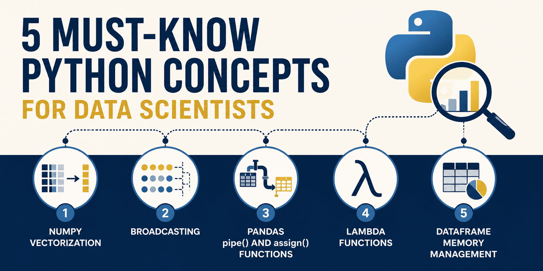
To put in writing high-performance knowledge programs, an information scientist should shift from customary procedural coding patterns to specialised, vectorized, and memory-aware approaches. On this article, we are going to dive deep into 5 must-know Python ideas that may enable you transition from writing clunky, sluggish spaghetti code to setting up lightning-fast, production-grade, and superbly practical knowledge pipelines.
# 1. NumPy Vectorization
Commonplace Python loops are sluggish. As a result of Python is an interpreted language, every iteration of a for loop incurs vital overhead: sort checking, dynamic methodology lookup, and reference counting. If you end up processing hundreds of thousands of information factors, these micro-overhead prices compound into multi-second bottlenecks.
The answer is NumPy vectorization. As an alternative of processing parts sequentially in Python bytecode, NumPy offloads loops to extremely optimized, pre-compiled C-extensions. These operations act on complete arrays without delay, executing contiguous array blocks on the machine degree, typically using Single Instruction, A number of Information (SIMD) directions.
// The Clunky Approach
Suppose now we have an inventory of 1 million float values representing uncooked sensor readings, and we have to scale every studying by 1.5 and apply a calibration fixed of 10.0. Utilizing an iterative Python loop:
import time

# A big checklist of 10 million sensor readings
n_elements = 10_000_000
data_list = [float(x) for x in range(n_elements)]

# Scaling values utilizing an specific python loop
start_time = time.time()
scaled_list = []

for val in data_list:
    scaled_list.append(val * 1.5 + 10.0)

loop_duration = time.time() - start_time

print(f"Loop implementation took: {loop_duration:.6f} seconds")
Output:
Loop implementation took: 0.378866 seconds
// The Vectorized Approach
Right here is the elegant, vectorized various. We load the info right into a contiguous NumPy array and carry out the arithmetic immediately on the array object:
import numpy as np
import time

# A big checklist of 10 million sensor readings
n_elements = 10_000_000

# Vectorized manner: NumPy performs the whole calculation in pre-compiled C loops
data_array = np.arange(n_elements, dtype=float)

start_time = time.time()
scaled_array = data_array * 1.5 + 10.0
numpy_duration = time.time() - start_time

print(f"NumPy implementation took: {numpy_duration:.6f} seconds")
print(f"Speedup: {loop_duration / numpy_duration:.1f}x sooner!")
Output:
Loop implementation took: 0.348456 seconds
NumPy implementation took: 0.013395 seconds
Speedup: 26.0x sooner!
By vectorizing the arithmetic, we are able to obtain a large efficiency increase with cleaner, extra concise code. The loop is eradicated from Python area and executed completely in high-speed C area.
# 2. Broadcasting: Math Guidelines for Mismatched Dimensions
In linear algebra, matrix operations typically require each operands to have the very same form. Nevertheless, in knowledge science, we frequently have to carry out operations on arrays of differing dimensions, resembling subtracting function column averages from a dataset, or normalizing row values.
Slightly than duplicating knowledge to drive matching shapes, NumPy makes use of a set of mathematical guidelines referred to as broadcasting. Broadcasting permits element-wise operations on arrays of various shapes by just about increasing the smaller array alongside the lacking or single-element dimensions, with out copying any knowledge in reminiscence.
The broadcasting guidelines are:
- If the arrays would not have the identical rank (variety of dimensions), prepend the form of the lower-rank array with 1s till each shapes have the identical size
- Two dimensions are suitable if they’re equal, or if certainly one of them is 1
- If suitable, the array behaves as if it had been stretched alongside the dimension of dimension 1 to match the opposite array’s form
// The Clunky Approach
Suppose now we have a 3×4 function matrix (3 samples, 4 options) and wish to subtract the column means to “de-mean” the options:
import numpy as np

options = np.array([
    [10.0, 20.0, 30.0, 4.0],
    [12.0, 24.0, 36.0, 8.0],
    [14.0, 28.0, 42.0, 12.0]
])

# Imply of every function column (form: (4,))
col_means = np.imply(options, axis=0)

# Utilizing nested loops to manually de-mean
demeaned_clunky = np.zeros_like(options)
for idx in vary(options.form[0]):
    for col_idx in vary(options.form[1]):
        demeaned_clunky[idx, col_idx] = options[idx, col_idx] - col_means[col_idx]

# Different: tiling the array to drive matching shapes
tiled_means = np.tile(col_means, (options.form[0], 1))
demeaned_tiled = options - tiled_means
// The Pythonic Approach
With broadcasting, we carry out the subtraction immediately. NumPy routinely aligns the (3, 4) function matrix with the (4,) column imply array by treating the column imply form as (1, 4):
import numpy as np

options = np.array([
    [10.0, 20.0, 30.0, 4.0],
    [12.0, 24.0, 36.0, 8.0],
    [14.0, 28.0, 42.0, 12.0]
])

col_means = np.imply(options, axis=0)

# Pythonic subtraction through computerized broadcasting
demeaned_broadcasting = options - col_means

# Dividing every row by its row sum
# row_sums has form (3,) -> to divide (3, 4) by (3,), we increase form to (3, 1) utilizing np.newaxis
row_sums = np.sum(options, axis=1)
normalized_features = options / row_sums[:, np.newaxis]

print("Demeaned:n", demeaned_broadcasting)
print("nNormalized Rows:n", normalized_features)
Output:
Demeaned:
 [[-2. -4. -6. -4.]
 [ 0.  0.  0.  0.]
 [ 2.  4.  6.  4.]]

Normalized Rows:
 [[0.15625    0.3125     0.46875    0.0625    ]
 [0.15       0.3        0.45       0.1       ]
 [0.14583333 0.29166667 0.4375     0.125     ]]
Broadcasting eliminates duplicate values and reminiscence copying. Below the hood, NumPy runs the subtraction loops at C pace with out making a tiled intermediate matrix, preserving reminiscence bandwidth and accelerating operations.
# 3. The Pandas .pipe() and .assign() Strategies: Clear, Useful Pipelines
Information preparation in Pandas typically degenerates into sequential spaghetti code. Builders create a number of intermediate DataFrames (df1, df2, and so forth.), modify variables in-place, or chain brackets. This results in code that’s troublesome to learn, onerous to check, and notoriously vulnerable to the dreaded SettingWithCopyWarning.
Trendy Pandas encourages transferring away from procedural mutations towards practical, declarative knowledge pipelines. By using .assign() for function creation and .pipe() for reusable multi-column operations, you’ll be able to chain steps in a single pipeline.
// The Clunky Approach
Let’s take a uncooked buyer gross sales dataset that requires filtering outliers, standardizing strings, imputing values, and calculating gross sales taxes.
import pandas as pd
import numpy as np

raw_data = {
    'Customer_ID': [101, 102, 103, 104, 105],
    'Age': [25, -5, 47, 120, 31],
    'Nation': ['usa', 'CANADA', 'usa', 'Germany', 'canada'],
    'Raw_Spend': [120.50, 450.00, 80.00, np.nan, 300.00]
}
df = pd.DataFrame(raw_data)

# Sequential intermediate mutations
df_clean = df.copy()

# 1. Filter out invalid ages
df_clean = df_clean[(df_clean['Age'] >= 0) & (df_clean['Age'] <= 100)]

# 2. Standardize nation names (dangers copy warnings)
df_clean['Country'] = df_clean['Country'].str.higher().str.strip()

# 3. Impute lacking Raw_Spend values
median_spend = df_clean['Raw_Spend'].median()
df_clean['Raw_Spend'] = df_clean['Raw_Spend'].fillna(median_spend)

# 4. Calculate Taxed_Spend
df_clean['Taxed_Spend'] = df_clean['Raw_Spend'] * 1.15

# 5. Format Column Names
df_clean = df_clean.rename(columns={'Customer_ID': 'customer_id'})
// The Pythonic Approach
Approaching this as a practical methodology chaining downside, we are able to wrap the nation standardization step right into a reusable utility operate and assemble a single, clear, self-contained pipeline.
import pandas as pd
import numpy as np

raw_data = {
    'Customer_ID': [101, 102, 103, 104, 105],
    'Age': [25, -5, 47, 120, 31],
    'Nation': ['usa', 'CANADA', 'usa', 'Germany', 'canada'],
    'Raw_Spend': [120.50, 450.00, 80.00, np.nan, 300.00]
}
df = pd.DataFrame(raw_data)

# Reusable customized transformation operate for .pipe()
def standardize_countries(dataframe: pd.DataFrame) -> pd.DataFrame:
    df_out = dataframe.copy()
    df_out['Country'] = df_out['Country'].str.higher().str.strip()
    return df_out

# Single elegant practical pipeline
df_clean_pipeline = (
    df.question("Age >= 0 and Age <= 100")
      .assign(
          Raw_Spend=lambda x: x['Raw_Spend'].fillna(x['Raw_Spend'].median()),
          Taxed_Spend=lambda x: x['Raw_Spend'] * 1.15
      )
      .pipe(standardize_countries)
      .rename(columns={'Customer_ID': 'customer_id'})
)

print(df_clean_pipeline)
Output:
   customer_id  Age Nation  Raw_Spend  Taxed_Spend
0          101   25     USA      120.5     138.5750
2          103   47     USA       80.0      92.0000
4          105   31  CANADA      300.0     345.0000
Methodology chaining ensures that the state of your unique DataFrame is rarely by chance mutated, stopping side-effects. .assign() handles column assignments by receiving a lambda operate the place x refers back to the lively state of the DataFrame at that time within the chain, whereas .pipe() permits customized operations to be cleanly modularized.
# 4. Lambda Capabilities for Information Transforms
Characteristic engineering often calls for small, single-purpose transformations, resembling formatting strings, splitting values, or making use of conditional statements. Writing customized named capabilities (utilizing def) for these easy calculations provides pointless boilerplate to your script.
A extra elegant method is utilizing lambda capabilities inside Pandas’ .map() and .apply(). Lambda capabilities are nameless, throwaway capabilities outlined on-the-fly with out a identify, good for fast knowledge mapping and clear inline transformations.
// The Clunky Approach
Suppose now we have a dataset of workers, and we have to map their distant work standing and parse their final names. A standard mistake is writing guide loops or using iterrows():
import pandas as pd

df = pd.DataFrame({
    'employee_name': ['john doe', 'jane smith', 'bob johnson'],
    'department_code': ['IT_01', 'HR_02', 'IT_03'],
    'is_remote': [1, 0, 1]
})

# Row-by-row iteration (sluggish and verbosely managed)
df_clunky = df.copy()
df_clunky['remote_status'] = None
df_clunky['last_name'] = None

for index, row in df_clunky.iterrows():
    # Parsing distant standing
    if row['is_remote'] == 1:
        df_clunky.at[index, 'remote_status'] = "Distant"
    else:
        df_clunky.at[index, 'remote_status'] = "Workplace"

    # Parsing and capitalizing final identify
    name_parts = row['employee_name'].break up()
    df_clunky.at[index, 'last_name'] = name_parts[1].capitalize()
// The Pythonic Approach
Right here is the clear, declarative method utilizing inline lambda transformations. We apply inline nameless logic to remodel columns immediately utilizing .map() for easy conversions and .apply() for customized string operations:
import pandas as pd

df = pd.DataFrame({
    'employee_name': ['john doe', 'jane smith', 'bob johnson'],
    'department_code': ['IT_01', 'HR_02', 'IT_03'],
    'is_remote': [1, 0, 1]
})

# Lambdas nested inside map() and apply()
df_opt = df.assign(
    remote_status=lambda d: d['is_remote'].map(lambda val: "Distant" if val == 1 else "Workplace"),
    last_name=lambda d: d['employee_name'].apply(lambda identify: identify.break up()[-1].capitalize()),
    dept_level=lambda d: d['department_code'].apply(lambda code: code.break up('_')[-1])
)

print(df_opt[['employee_name', 'last_name', 'remote_status', 'dept_level']])
Output:
  employee_name last_name remote_status dept_level
0      john doe       Doe        Distant         01
1    jane smith     Smith        Workplace         02
2   bob johnson   Johnson        Distant         03
Utilizing lambdas lets you write self-contained transformations that preserve your logic tightly sure to the column creation statements. By combining lambda with .map() and .apply(), you remove verbose nested loops and preserve your code superbly readable.
# 5. Reminiscence Administration with DataFrames: Optimizing dtypes
By default, when Pandas imports a dataset (e.g. from CSV or database information), it performs it secure. Integers are loaded as 64-bit (int64), decimals as 64-bit (float64), and textual content columns as generic object varieties. Whereas secure, this defaults to most reminiscence footprint. A dataset of just a few hundred thousand rows can shortly devour gigabytes of system RAM, resulting in native slow-downs or “out of reminiscence” errors on manufacturing servers.
We will drastically scale back a DataFrame’s reminiscence footprint by downcasting numeric columns to smaller integers/floats and changing low-cardinality textual content columns to class knowledge varieties.
For example, an age column has values starting from 0 to 100, which may simply slot in a single 8-bit integer (int8, which holds values as much as 127) reasonably than the usual 64-bit (int64) datatype. Equally, class values map textual content strings to easy integer codes below the hood, yielding huge area financial savings.
// The Clunky Approach
Let’s generate an artificial subscriber dataset of 100,000 customers and take a look at the reminiscence consumed by default Pandas varieties:
import pandas as pd
import numpy as np

n_rows = 100_000
np.random.seed(42)

df_large = pd.DataFrame({
    'user_id': np.random.randint(1000000, 1000000 + n_rows, dimension=n_rows),
    'age': np.random.randint(18, 90, dimension=n_rows),
    'device_type': np.random.alternative(['iOS', 'Android', 'Web', 'SmartTV'], dimension=n_rows),
    'monthly_revenue': np.random.uniform(5.0, 150.0, dimension=n_rows),
    'active_subscriber': np.random.alternative([0, 1], dimension=n_rows)
})

# Inspecting reminiscence utilization
print(df_large.information(memory_usage="deep"))
memory_before = df_large.memory_usage(deep=True).sum() / (1024 ** 2)
print(f"Default Reminiscence Utilization: {memory_before:.2f} MB")
Output:
RangeIndex: 100000 entries, 0 to 99999
Information columns (complete 5 columns):
 #   Column             Non-Null Rely   Dtype
---  ------             --------------   -----
 0   user_id            100000 non-null  int64
 1   age                100000 non-null  int64
 2   device_type        100000 non-null  object
 3   monthly_revenue    100000 non-null  float64
 4   active_subscriber  100000 non-null  int64
dtypes: float64(1), int64(3), object(1)
reminiscence utilization: 8.2 MB
None
Default Reminiscence Utilization: 8.20 MB
// The Pythonic Approach
Now let’s apply our optimizations: casting columns to their minimal required numeric bounds and changing textual content columns to class:
# Downcasting varieties
df_optimized = df_large.assign(
    user_id=df_large['user_id'].astype('int32'),                    # Max 1.1 million matches in int32
    age=df_large['age'].astype('int8'),                             # Max age 90 matches in int8
    device_type=df_large['device_type'].astype('class'),         # Low cardinality (4 distinctive strings)
    monthly_revenue=df_large['monthly_revenue'].astype('float32'),  # Single precision float is a lot
    active_subscriber=df_large['active_subscriber'].astype('int8')  # Binary flag matches in int8
)

# Inspecting optimized reminiscence utilization
print(df_optimized.information(memory_usage="deep"))
memory_after = df_optimized.memory_usage(deep=True).sum() / (1024 ** 2)

print(f"Optimized Reminiscence Utilization: {memory_after:.2f} MB")
print(f"Reminiscence Footprint Discount: {((memory_before - memory_after) / memory_before) * 100:.1f}%")
Output:
reminiscence utilization: 1.0 MB
None
Optimized Reminiscence Utilization: 1.05 MB
Reminiscence Footprint Discount: 87.2%
By merely adjusting our column dtypes, we shrank the DataFrame’s dimension by almost 90%! Through the use of class for low-cardinality strings, Pandas avoids duplicating character strings throughout rows, mapping every row to a light-weight integer index as an alternative.
# Wrapping Up
Mastering these 5 elementary Python ideas is a big step towards changing into a senior knowledge scientist who designs environment friendly, readable, and extremely optimized knowledge pipelines.
By leveraging vectorization and broadcasting in NumPy, you remove uncooked Python loops and unlock hardware-level speedups. Shifting to practical Pandas pipelines with .pipe() and .assign() elevates the readability and security of your feature-engineering workflows. Combining these with inline lambda capabilities for on-the-fly transformations and proactive reminiscence administration via dtypes lets you scale your algorithms from native prototypes to very large manufacturing workloads seamlessly.
Information science is as a lot about software program engineering as it’s about arithmetic. Deal with your code as a first-class product, and your datasets will course of sooner, your pipelines will fail much less, and your programs will likely be a pleasure to construct.
You’ll want to try the earlier articles on this sequence:
Matthew Mayo (@mattmayo13) holds a grasp’s diploma in laptop science and a graduate diploma in knowledge mining. As managing editor of KDnuggets & Statology, and contributing editor at Machine Studying Mastery, Matthew goals to make complicated knowledge science ideas accessible. His skilled pursuits embrace pure language processing, language fashions, machine studying algorithms, and exploring rising AI. He’s pushed by a mission to democratize data within the knowledge science group. Matthew has been coding since he was 6 years previous.


