


have been first launched for pictures, and for pictures they’re typically straightforward to know.
A filter slides over pixels and detects edges, shapes, or textures. You possibly can learn this text I wrote earlier to know how CNNs work for pictures with Excel.
For textual content, the concept is identical.
As a substitute of pixels, we slide filters over phrases.
As a substitute of visible patterns, we detect linguistic patterns.
And plenty of vital patterns in textual content are very native. Let’s take these quite simple examples:
- “good” is constructive
- “unhealthy” is detrimental
- “not good” is detrimental
- “not unhealthy” is usually constructive
In my earlier article, we noticed the right way to characterize phrases as numbers utilizing embeddings.
We additionally noticed a key limitation: after we used a worldwide common, phrase order was utterly ignored.
From the mannequin’s viewpoint, “not good” and “good not” seemed precisely the identical.
So the following problem is obvious: we would like the mannequin to take phrase order under consideration.
A 1D Convolutional Neural Community is a pure software for this, as a result of it scans a sentence with small sliding home windows and reacts when it acknowledges acquainted native patterns.
1. Understanding a 1D CNN for Textual content: Structure and Depth
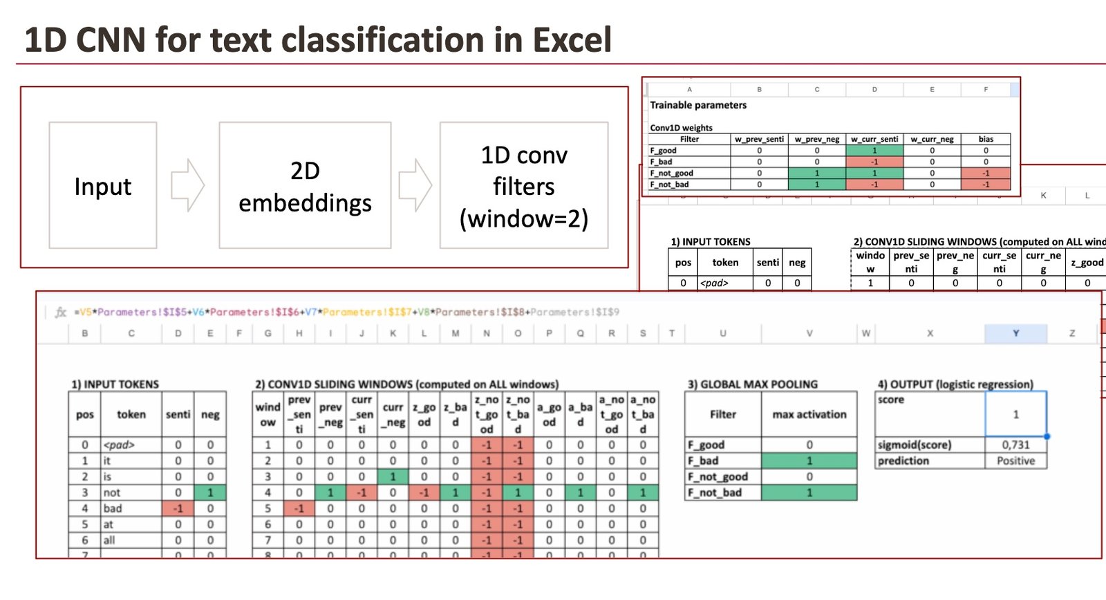
1.1. Constructing a 1D CNN for textual content in Excel
On this article, we construct a 1D CNN structure in Excel with the next parts:
- Embedding dictionary
We use a 2-dimensional embedding. As a result of one dimension just isn’t sufficient for this process.
One dimension encodes sentiment, and the second dimension encodes negation. - Conv1D layer
That is the core part of a CNN structure.
It consists of filters that slide throughout the sentence with a window size of two phrases. We select 2 phrases to be easy. - ReLU and world max pooling
These steps hold solely the strongest matches detected by the filters.
We can even focus on the truth that ReLU is non-compulsory. - Logistic regression
That is the ultimate classification layer, which mixes the detected patterns right into a chance.

This pipeline corresponds to a typical CNN textual content classifier.
The one distinction right here is that we explicitly write and visualize the ahead cross in Excel.
1.2. What “deep studying” means on this structure
Earlier than going additional, allow us to take a step again.
Sure, I do know, I do that typically, however having a worldwide view of fashions actually helps to know them.
The definition of deep studying is usually blurred.
For many individuals, deep studying merely means “many layers”.
Right here, I’ll take a barely completely different viewpoint.
What actually characterizes deep studying just isn’t the variety of layers, however the depth of the transformation utilized to the enter knowledge.
With this definition:
- Even a mannequin with a single convolution layer might be thought of deep studying,
- as a result of the enter is reworked right into a extra structured and summary illustration.
Alternatively, taking uncooked enter knowledge, making use of one-hot encoding, and stacking many totally linked layers doesn’t essentially make a mannequin deep in a significant sense.
In concept, if we don’t have any transformation, one layer is sufficient.
In CNNs, the presence of a number of layers has a really concrete motivation.
Contemplate a sentence like:
This film just isn’t excellent
With a single convolution layer and a small window, we are able to detect easy native patterns comparable to: “very + good”
However we can not but detect higher-level patterns comparable to: “not + (excellent)”
This is the reason CNNs are sometimes stacked:
- the primary layer detects easy native patterns,
- the second layer combines them into extra advanced ones.
On this article, we intentionally concentrate on one convolution layer.
This makes each step seen and simple to know in Excel, whereas holding the logic equivalent to deeper CNN architectures.
2. Turning phrases into embeddings
Allow us to begin with some easy phrases. We are going to attempt to detect negation, so we’ll use these phrases, with different phrases (that we’ll not mannequin)
- “good”
- “unhealthy”
- “not good”
- “not unhealthy”
We hold the illustration deliberately small so that each step is seen.
We are going to solely use a dictionary of three phrases : good, unhealthy and never.
All different phrases could have 0 as embeddings.
2.1 Why one dimension just isn’t sufficient
In a earlier article on sentiment detection, we used a single dimension.
That labored for “good” versus “unhealthy”.
However now we need to deal with negation.
One dimension can solely characterize one idea nicely.
So we want two dimensions:
- senti: sentiment polarity
- neg: negation marker
2.2 The embedding dictionary
Every phrase turns into a 2D vector:
- good → (senti = +1, neg = 0)
- unhealthy → (senti = -1, neg = 0)
- not → (senti = 0, neg = +1)
- another phrase → (0, 0)

This isn’t how actual embeddings look. Actual embeddings are realized, high-dimensional, and never straight interpretable.
However for understanding how Conv1D works, this toy embedding is ideal.
In Excel, that is only a lookup desk.
In an actual neural community, this embedding matrix can be trainable.

3. Conv1D filters as sliding sample detectors
Now we arrive on the core concept of a 1D CNN.
A Conv1D filter is nothing mysterious. It’s only a small set of weights plus a bias that slides over the sentence.
As a result of:
- every phrase embedding has 2 values (senti, neg)
- our window comprises 2 phrases
every filter has:
- 4 weights (2 dimensions × 2 positions)
- 1 bias
That’s all.
You possibly can consider a filter as repeatedly asking the identical query at each place:
“Do these two neighboring phrases match a sample I care about?”
3.1 Sliding home windows: how Conv1D sees a sentence
Contemplate this sentence:
it’s not unhealthy in any respect
We select a window dimension of two phrases.
Meaning the mannequin appears to be like at each adjoining pair:
- (it, is)
- (is, not)
- (not, unhealthy)
- (unhealthy, at)
- (at, all)
Necessary level:
The filters slide in every single place, even when each phrases are impartial (all zeros).

3.2 4 intuitive filters
To make the conduct straightforward to know, we use 4 filters.

Filter 1 – “I see GOOD”
This filter appears to be like solely on the sentiment of the present phrase.
Plain-text equation for one window:
z = senti(current_word)
If the phrase is “good”, z = 1
If the phrase is “unhealthy”, z = -1
If the phrase is impartial, z = 0
After ReLU, detrimental values turn into 0. However it’s non-compulsory.
Filter 2 – “I see BAD”
This one is symmetric.
z = -senti(current_word)
So:
- “unhealthy” → z = 1
- “good” → z = -1 → ReLU → 0
Filter 3 – “I see NOT GOOD”
This filter appears to be like at two issues on the identical time:
- neg(previous_word)
- senti(current_word)
Equation:
z = neg(previous_word) + senti(current_word) – 1
Why the “-1”?
It acts like a threshold in order that each situations should be true.
Outcomes:
- “not good” → 1 + 1 – 1 = 1 → activated
- “is nice” → 0 + 1 – 1 = 0 → not activated
- “not unhealthy” → 1 – 1 – 1 = -1 → ReLU → 0
Filter 4 – “I see NOT BAD”
Identical concept, barely completely different signal:
z = neg(previous_word) + (-senti(current_word)) – 1
Outcomes:
- “not unhealthy” → 1 + 1 – 1 = 1
- “not good” → 1 – 1 – 1 = -1 → 0
This can be a crucial instinct:
A CNN filter can behave like a native logical rule, realized from knowledge.
3.3 Remaining results of sliding home windows
Right here is the ultimate outcomes of those 4 filters.

4. ReLU and max pooling: from native to world
4.1 ReLU
After computing z for each window, we apply ReLU:
ReLU(z) = max(0, z)
That means:
- detrimental proof is ignored
- constructive proof is stored
Every filter turns into a presence detector.
By the best way, it’s an activation operate within the Neural community. So a Neural community just isn’t that tough in spite of everything.
4.2 World Max pooling
Then comes world max pooling.
For every filter, we hold solely:
max activation over all home windows
Interpretation:
“I don’t care the place the sample seems, solely whether or not it seems strongly someplace.”
At this level, the entire sentence is summarized by 4 numbers:
- strongest “good” sign
- strongest “unhealthy” sign
- strongest “not good” sign
- strongest “not unhealthy” sign

4.3 What occurs if we take away ReLU?
With out ReLU:
- detrimental values keep detrimental
- max pooling might choose detrimental values
This mixes two concepts:
- absence of a sample
- reverse of a sample
The filter stops being a clear detector and turns into a signed rating.
The mannequin may nonetheless work mathematically, however interpretation turns into more durable.
5. The ultimate layer is logistic regression
Now we mix these indicators.
We compute a rating utilizing a linear mixture:
rating = 2 × F_good – 2 × F_bad – 3 × F_not_good – 3 × F_not_bad – bias

Then we convert the rating right into a chance:
chance = 1 / (1 + exp(-score))
That’s precisely logistic regression.
So sure:
- the CNN extracts options: this step might be thought of as function engineering, proper?
- logistic regression makes the ultimate choices, it’s a traditional machine studying mannequin we all know nicely

6. Full examples with sliding filters
Instance 1
“it’s unhealthy, so it’s not good in any respect”
The sentence comprises:
After max pooling:
- F_good = 1 (as a result of “good” exists)
- F_bad = 1
- F_not_good = 1
- F_not_bad = 0
Remaining rating turns into strongly detrimental.
Prediction: detrimental sentiment.

Instance 2
“it’s good. sure, not unhealthy.”
The sentence comprises:
After max pooling:
- F_good = 1
- F_bad = 1 (as a result of the phrase “unhealthy” seems)
- F_not_good = 0
- F_not_bad = 1
The ultimate linear layer learns that “not unhealthy” ought to outweigh “unhealthy”.
Prediction: constructive sentiment.
This additionally exhibits one thing vital: max pooling retains all sturdy indicators.
The ultimate layer decides the right way to mix them.

Exemple 3 with A limitation that explains why CNNs get deeper
Do that sentence:
“it’s not very unhealthy”
With a window of dimension 2, the mannequin sees:
It by no means sees (not, unhealthy), so the “not unhealthy” filter by no means fires.
It explains why actual fashions use:
- bigger home windows
- a number of convolution layers
- or different architectures for longer dependencies
Conclusion
The energy of Excel is visibility.
You possibly can see:
- the embedding dictionary
- all filter weights and biases
- each sliding window
- each ReLU activation
- the max pooling end result
- the logistic regression parameters
Coaching is just the method of adjusting these numbers.
When you see that, CNNs cease being mysterious.
They turn into what they are surely: structured, trainable sample detectors that slide over knowledge.


