


With Logistic Regression, we realized the right way to classify into two courses.
Now, what occurs if there are greater than two courses.
n is just the multiclass extension of this concept. And we’ll focus on this mannequin for Day 14 of my Machine Studying “Creation Calendar” (comply with this hyperlink to get all of the details about the strategy and the information I exploit).
As an alternative of 1 rating, we now create one rating per class. As an alternative of 1 chance, we apply the Softmax perform to supply possibilities that sum to 1.
Understanding the Softmax mannequin
Earlier than coaching the mannequin, allow us to first perceive what the mannequin is.
Softmax Regression just isn’t about optimization but.
It’s first about how predictions are computed.
A tiny dataset with 3 courses
Allow us to use a small dataset with one characteristic x and three courses.
As we stated earlier than, the goal variable y ought to not be handled as numerical.
It represents classes, not portions.
A typical solution to signify that is one-hot encoding, the place every class is represented by its personal indicator.
From this viewpoint, Softmax Regression might be seen as three Logistic Regressions operating in parallel, one per class.
Small datasets are perfect for studying.
You’ll be able to see each system, each worth, and the way every a part of the mannequin contributes to the ultimate end result.

Description of the Mannequin
So what’s the mannequin, precisely?
Rating per class
In logistic regression, the mannequin rating is an easy linear expression: rating = a * x + b.
Softmax Regression does precisely the identical, however one rating per class:
score_0 = a0 * x + b0
score_1 = a1 * x + b1
score_2 = a2 * x + b2
At this stage, these scores are simply actual numbers.
They aren’t possibilities but.
Turning scores into possibilities: the Softmax step
Softmax converts the three scores into three possibilities. Every chance is optimistic, and all three sum to 1.
The computation is direct:
- Exponentiate every rating
- Compute the sum of all exponentials
- Divide every exponential by this sum
This offers us p0, p1, and p2 for every row.
These values signify the mannequin confidence for every class.
At this level, the mannequin is absolutely outlined.
Coaching the mannequin will merely consist in adjusting the coefficients ak and bk in order that these possibilities match the noticed courses in addition to potential.

Visualizing the Softmax mannequin
At this level, the mannequin is absolutely outlined.
We’ve:
- one linear rating per class
- a Softmax step that turns these scores into possibilities
Coaching the mannequin merely consists in adjusting the coefficients aka_kak and bkb_kbk in order that these possibilities match the noticed courses in addition to potential.
As soon as the coefficients have been discovered, we will visualize the mannequin habits.
To do that, we take a spread of enter values, for instance x from 0 to 7, and we compute: score0,score1,score2 and the corresponding possibilities p0,p1,p2.
Plotting these possibilities provides three easy curves, one per class.

The end result could be very intuitive.
For small values of x, the chance of sophistication 0 is excessive.
As x will increase, this chance decreases, whereas the chance of sophistication 1 will increase.
For bigger values of x, the chance of sophistication 2 turns into dominant.
At each worth of x, the three possibilities sum to 1.
The mannequin doesn’t make abrupt choices; as an alternative, it expresses how assured it’s in every class.
This plot makes the habits of Softmax Regression simple to grasp.
- You’ll be able to see how the mannequin transitions easily from one class to a different
- Determination boundaries correspond to intersections between chance curves
- The mannequin logic turns into seen, not summary
This is without doubt one of the key advantages of constructing the mannequin in Excel:
you don’t simply compute predictions, you’ll be able to see how the mannequin thinks.
Now that the mannequin is outlined, we’d like a solution to consider how good it’s, and a technique to enhance its coefficients.
Each steps reuse concepts we already noticed with Logistic Regression.
Evaluating the mannequin: Cross-Entropy Loss
Softmax Regression makes use of the identical loss perform as Logistic Regression.
For every information level, we have a look at the chance assigned to the right class, and we take the destructive logarithm:
loss = – log (p true class)
If the mannequin assigns a excessive chance to the right class, the loss is small.
If it assigns a low chance, the loss turns into giant.
In Excel, that is quite simple to implement.
We choose the right chance based mostly on the worth of y, and apply the logarithm:
loss = -LN( CHOOSE(y + 1, p0, p1, p2) )
Lastly, we compute the common loss over all rows.
This common loss is the amount we wish to reduce.

Computing residuals
To replace the coefficients, we begin by computing residuals, one per class.
For every row:
- residual_0 = p0 minus 1 if y equals 0, in any other case 0
- residual_1 = p1 minus 1 if y equals 1, in any other case 0
- residual_2 = p2 minus 1 if y equals 2, in any other case 0
In different phrases, for the right class, we subtract 1.
For the opposite courses, we subtract 0.
These residuals measure how far the expected possibilities are from what we count on.
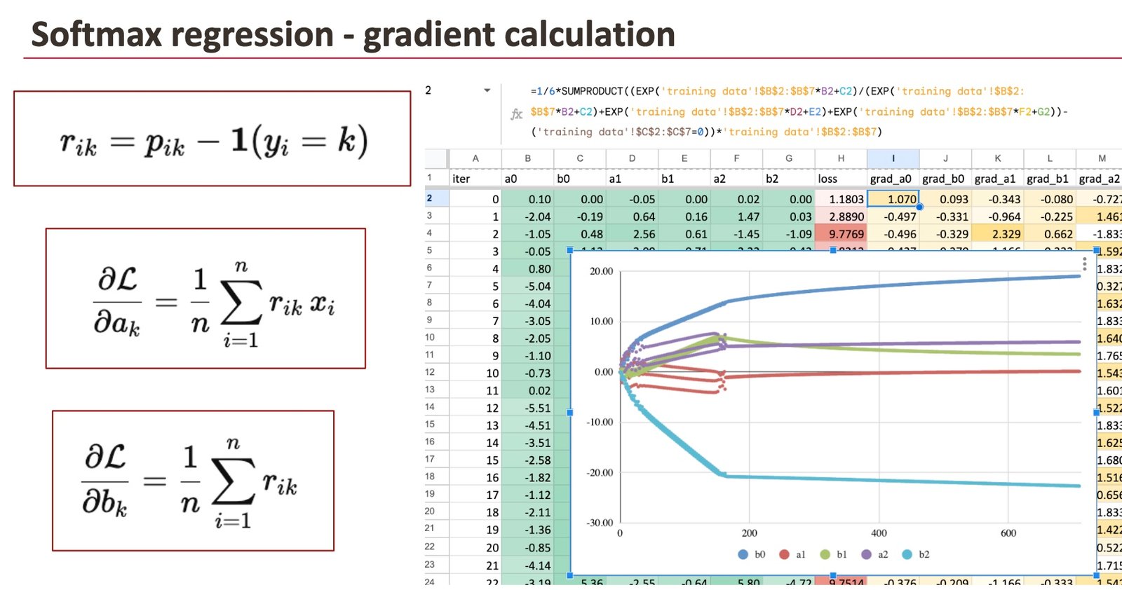
Computing the gradients
The gradients are obtained by combining the residuals with the characteristic values.
For every class okay:
- the gradient of ak is the typical of
residual_k * x - the gradient of bk is the typical of
residual_k
In Excel, that is applied with easy formulation equivalent to SUMPRODUCT and AVERAGE.
At this level, every thing is express:
you see the residuals, the gradients, and the way every information level contributes.

Updating the coefficients
As soon as the gradients are recognized, we replace the coefficients utilizing gradient descent.
This step is an identical as we noticed earlier than, fore Logistic Regression or Linear regression.
The one distinction is that we now replace six coefficients as an alternative of two.
To visualise studying, we create a second sheet with one row per iteration:
- the present iteration quantity
- the six coefficients (a0, b0, a1, b1, a2, b2)
- the loss
- the gradients
Row 2 corresponds to iteration 0, with the preliminary coefficients.
Row 3 computes the up to date coefficients utilizing the gradients from row 2.
By dragging the formulation down for a whole lot of rows, we simulate gradient descent over many iterations.
You’ll be able to then clearly see:
- the coefficients steadily stabilizing
- the loss lowering iteration after iteration
This makes the educational course of tangible.
As an alternative of imagining an optimizer, you’ll be able to watch the mannequin study.

Logistic Regression as a Particular Case of Softmax Regression
Logistic Regression and Softmax Regression are sometimes offered as totally different fashions.
In actuality, they’re the identical concept at totally different scales.
Softmax Regression computes one linear rating per class and turns these scores into possibilities by evaluating them.
When there are solely two courses, this comparability relies upon solely on the distinction between the 2 scores.
This distinction is a linear perform of the enter, and making use of Softmax on this case produces precisely the logistic (sigmoid) perform.
In different phrases, Logistic Regression is just Softmax Regression utilized to 2 courses, with redundant parameters eliminated.
As soon as that is understood, shifting from binary to multiclass classification turns into a pure extension, not a conceptual bounce.

Softmax Regression doesn’t introduce a brand new mind-set.
It merely exhibits that Logistic Regression already contained every thing we would have liked.
By duplicating the linear rating as soon as per class and normalizing them with Softmax, we transfer from binary choices to multiclass possibilities with out altering the underlying logic.
The loss is identical concept.
The gradients are the identical construction.
The optimization is identical gradient descent we already know.
What modifications is just the variety of parallel scores.
One other Technique to Deal with Multiclass Classification?
Softmax just isn’t the one solution to cope with multiclass issues in weight-based fashions.
There may be one other strategy, much less elegant conceptually, however quite common in follow:
one-vs-rest or one-vs-one classification.
As an alternative of constructing a single multiclass mannequin, we prepare a number of binary fashions and mix their outcomes.
This technique is used extensively with Help Vector Machines.
Tomorrow, we’ll have a look at SVM.
And you will note that it may be defined in a somewhat uncommon method… and, as traditional, immediately in Excel.


