


of my Machine Studying “Introduction Calendar”. I want to thanks in your assist.
I’ve been constructing these Google Sheet recordsdata for years. They advanced little by little. However when it’s time to publish them, I at all times want hours to reorganize all the things, clear the format, and make them nice to learn.
Right now, we transfer to DBSCAN.
DBSCAN Does Not Be taught a Parametric Mannequin
Identical to LOF, DBSCAN is not a parametric mannequin. There isn’t a system to retailer, no guidelines, no centroids, and nothing compact to reuse later.
We should maintain the entire dataset as a result of the density construction will depend on all factors.
Its full title is Density-Primarily based Spatial Clustering of Functions with Noise.
However cautious: this “density” isn’t a Gaussian density.
It’s a count-based notion of density. Simply “what number of neighbors dwell near me”.
Why DBSCAN Is Particular
As its title signifies, DBSCAN does two issues on the identical time:
- it finds clusters
- it marks anomalies (the factors that don’t belong to any cluster)
That is precisely why I current the algorithms on this order:
- ok-means and GMM are clustering fashions. They output a compact object: centroids for k-means, means and variances for GMM.
- Isolation Forest and LOF are pure anomaly detection fashions. Their solely aim is to search out uncommon factors.
- DBSCAN sits in between. It does each clustering and anomaly detection, primarily based solely on the notion of neighborhood density.
A Tiny Dataset to Hold Issues Intuitive
We stick with the identical tiny dataset that we used for LOF: 1, 2, 3, 7, 8, 12
For those who take a look at these numbers, you already see two compact teams:
one round 1–2–3, one other round 7–8, and 12 dwelling alone.
DBSCAN captures precisely this instinct.
Abstract in 3 Steps
DBSCAN asks three easy questions for every level:
- What number of neighbors do you have got inside a small radius (eps)?
- Do you have got sufficient neighbors to change into a Core level (minPts)?
- As soon as we all know the Core factors, to which related group do you belong?
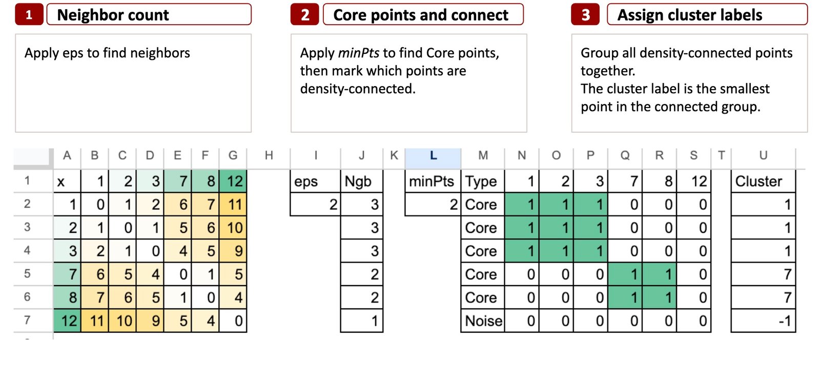
Right here is the abstract of the DBSCAN algorithm in 3 steps:

Allow us to start step-by-step.
DBSCAN in 3 steps
Now that we perceive the thought of density and neighborhoods, DBSCAN turns into very straightforward to explain.
Every little thing the algorithm does matches into three easy steps.
Step 1 – Rely the neighbors
The aim is to verify what number of neighbors every level has.
We take a small radius referred to as eps.
For every level, we take a look at all different factors and mark these whose distance is lower than eps.
These are the neighbors.
This offers us the primary thought of density:
some extent with many neighbors is in a dense area,
some extent with few neighbors lives in a sparse area.
For a 1-dimensional toy instance like ours, a standard selection is:
eps = 2
We draw just a little interval of radius 2 round every level.
Why is it referred to as eps?
The title eps comes from the Greek letter ε (epsilon), which is historically utilized in arithmetic to characterize a small amount or a small radius round some extent.
So in DBSCAN, eps is actually “the small neighborhood radius”.
It solutions the query:
How far do we glance round every level?
So in Excel, step one is to compute the pairwise distance matrix, then rely what number of neighbors every level has inside eps.

Step 2 – Core Factors and Density Connectivity
Now that we all know the neighbors from Step 1, we apply minPts to resolve which factors are Core.
minPts means right here minimal variety of factors.
It’s the smallest variety of neighbors some extent should have (contained in the eps radius) to be thought of a Core level.
Some extent is Core if it has a minimum of minPts neighbors inside eps.
In any other case, it might change into Border or Noise.
With eps = 2 and minPts = 2, we’ve 12 that’s not Core.
As soon as the Core factors are recognized, we merely verify which factors are density-reachable from them. If some extent might be reached by shifting from one Core level to a different inside eps, it belongs to the identical group.
In Excel, we will characterize this as a easy connectivity desk that exhibits which factors are linked by way of Core neighbors.
This connectivity is what DBSCAN makes use of to type clusters in Step 3.

Step 3 – Assign cluster labels
The aim is to show connectivity into precise clusters.
As soon as the connectivity matrix is prepared, the clusters seem naturally.
DBSCAN merely teams all related factors collectively.
To offer every group a easy and reproducible title, we use a really intuitive rule:
The cluster label is the smallest level within the related group.
For instance:
- Group {1, 2, 3} turns into cluster 1
- Group {7, 8} turns into cluster 7
- Some extent like 12 with no Core neighbors turns into Noise
That is precisely what we’ll show in Excel utilizing formulation.

Closing ideas
DBSCAN is ideal to show the thought of native density.
There isn’t a chance, no Gaussian system, no estimation step.
Simply distances, neighbors, and a small radius.
However this simplicity additionally limits it.
As a result of DBSCAN makes use of one mounted radius for everybody, it can’t adapt when the dataset accommodates clusters of various scales.
HDBSCAN retains the identical instinct, however seems at all radii and retains what stays steady.
It’s way more strong, and far nearer to how people naturally see clusters.


