


Introduction
My earlier posts seemed on the bog-standard choice tree and the marvel of a random forest. Now, to finish the triplet, I’ll visually discover !
There are a bunch of gradient boosted tree libraries, together with XGBoost, CatBoost, and LightGBM. Nonetheless, for this I’m going to make use of sklearn’s one. Why? Just because, in contrast with the others, it allowed me to visualise simpler. In follow I have a tendency to make use of the opposite libraries greater than the sklearn one; nevertheless, this venture is about visible studying, not pure efficiency.
Essentially, a GBT is a mix of bushes that solely work collectively. Whereas a single choice tree (together with one extracted from a random forest) could make a good prediction by itself, taking a person tree from a GBT is unlikely to present something usable.
Past this, as all the time, no principle, no maths — simply plots and hyperparameters. As earlier than, I’ll be utilizing the California housing dataset through scikit-learn (CC-BY), the identical basic course of as described in my earlier posts, the code is at https://github.com/jamesdeluk/data-projects/tree/important/visualising-trees, and all photos beneath are created by me (other than the GIF, which is from Tenor).
A fundamental gradient boosted tree
Beginning with a fundamental GBT: gb = GradientBoostingRegressor(random_state=42). Much like different tree varieties, the default settings for min_samples_split, min_samples_leaf, max_leaf_nodes are 2, 1, None respectively. Apparently, the default max_depth is 3, not None as it’s with choice bushes/random forests. Notable hyperparameters, which I’ll look into extra later, embrace learning_rate (how steep the gradient is, default 0.1), and n_estimators (just like random forest — the variety of bushes).
Becoming took 2.2s, predicting took 0.005s, and the outcomes:
| Metric | max_depth=None |
|---|---|
| MAE | 0.369 |
| MAPE | 0.216 |
| MSE | 0.289 |
| RMSE | 0.538 |
| R² | 0.779 |
So, faster than the default random forest, however barely worse efficiency. For my chosen block, it predicted 0.803 (precise 0.894).
Visualising
For this reason you’re right here, proper?
The tree
Much like earlier than, we are able to plot a single tree. That is the primary one, accessed with gb.estimators_[0, 0]:

I’ve defined these within the earlier posts, so I received’t achieve this once more right here. One factor I’ll carry to your consideration although: discover how horrible the values are! Three of the leaves even have adverse values, which we all know can’t be the case. For this reason a GBT solely works as a mixed ensemble, not as separate standalone bushes like in a random forest.
Predictions and errors
My favorite option to visualise GBTs is with prediction vs iteration plots, utilizing gb.staged_predict. For my chosen block:

Bear in mind the default mannequin has 100 estimators? Properly, right here they’re. The preliminary prediction was method off — 2! However every time it learnt (bear in mind learning_rate?), and bought nearer to the actual worth. In fact, it was educated on the coaching knowledge, not this particular knowledge, so the ultimate worth was off (0.803, so about 10% off), however you’ll be able to clearly see the method.
On this case, it reached a reasonably regular state after about 50 iterations. Later we’ll see easy methods to cease iterating at this stage, to keep away from losing money and time.
Equally, the error (i.e. the prediction minus the true worth) will be plotted. In fact, this provides us the identical plot, merely with completely different y-axis values:

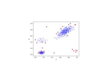
Let’s take this one step additional! The check knowledge has over 5000 blocks to foretell; we are able to loop by way of every, and predict all of them, for every iteration!

I like this plot.

All of them begin round 2, however explode throughout the iterations. We all know all of the true values fluctuate from 0.15 to five, with a imply of two.1 (verify my first put up), so this spreading out of predictions (from ~0.3 to ~5.5) is as anticipated.
We will additionally plot the errors:

At first look, it appears a bit unusual — we’d anticipate them to begin at, say, ±2, and converge on 0. Trying fastidiously although, this does occur for many — it may be seen within the left-hand facet of the plot, the primary 10 iterations or so. The issue is, with over 5000 traces on this plot, there are quite a lot of overlapping ones, making the outliers stand out extra. Maybe there’s a greater option to visualise these? How about…

The median error is 0.05 — which is excellent! The IQR is lower than 0.5, which can also be first rate. So, whereas there are some horrible predictions, most are first rate.
Hyperparameter tuning
Choice tree hyperparameters
Similar as earlier than, let’s evaluate how the hyperparameters explored within the authentic choice tree put up apply to GBTs, with the default hyperparameters of learning_rate = 0.1, n_estimators = 100. The min_samples_leaf, min_samples_split, and max_leaf_nodes one even have max_depth = 10, to make it a good comparability to earlier posts and to one another.
| Mannequin | max_depth=None | max_depth=10 | min_samples_leaf=10 | min_samples_split=10 | max_leaf_nodes=100 |
|---|---|---|---|---|---|
| Match Time (s) | 10.889 | 7.009 | 7.101 | 7.015 | 6.167 |
| Predict Time (s) | 0.089 | 0.019 | 0.015 | 0.018 | 0.013 |
| MAE | 0.454 | 0.304 | 0.301 | 0.302 | 0.301 |
| MAPE | 0.253 | 0.177 | 0.174 | 0.174 | 0.175 |
| MSE | 0.496 | 0.222 | 0.212 | 0.217 | 0.210 |
| RMSE | 0.704 | 0.471 | 0.46 | 0.466 | 0.458 |
| R² | 0.621 | 0.830 | 0.838 | 0.834 | 0.840 |
| Chosen Prediction | 0.885 | 0.906 | 0.962 | 0.918 | 0.923 |
| Chosen Error | 0.009 | 0.012 | 0.068 | 0.024 | 0.029 |
Not like choice bushes and random forests, the deeper tree carried out far worse! And took longer to suit. Nonetheless, rising the depth from 3 (the default) to 10 has improved the scores. The opposite constraints resulted in additional enhancements — once more displaying how all hyperparameters can play a task.
learning_rate
GBTs function by tweaking predictions after every iteration primarily based on the error. The upper the adjustment (a.okay.a. the gradient, a.okay.a. the training price), the extra the prediction modifications between iterations.
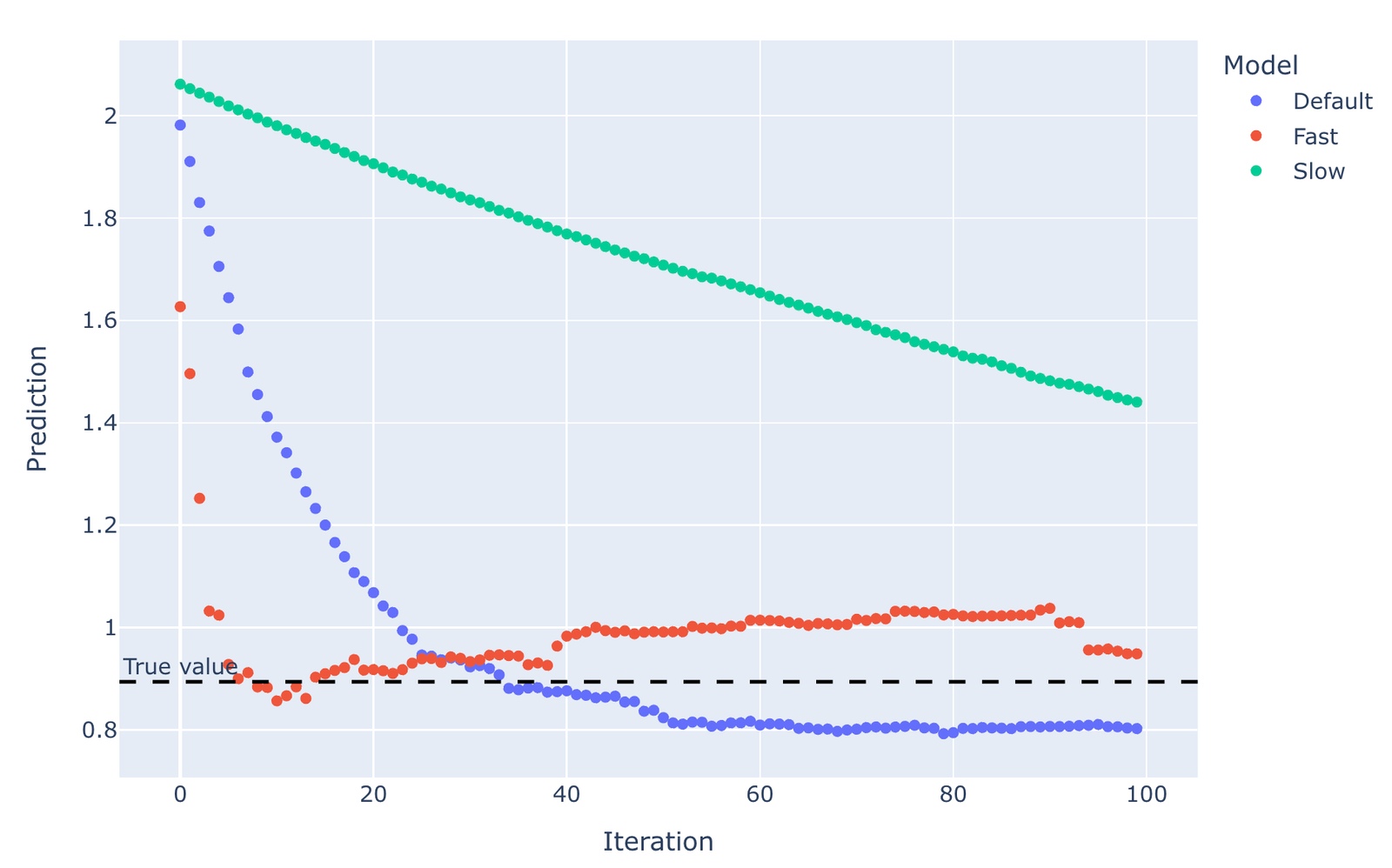
There’s a clear trade-off for studying price. Evaluating studying charges of 0.01 (Sluggish), 0.1 (Default), and 0.5 (Quick), over 100 iterations:

Quicker studying charges can get to the right worth faster, however they’re extra prone to overcorrect and soar previous the true worth (suppose fishtailing in a automobile), and may result in oscillations. Sluggish studying charges could by no means attain the right worth (suppose… not turning the steering wheel sufficient and driving straight right into a tree). As for the stats:
| Mannequin | Default | Quick | Sluggish |
|---|---|---|---|
| Match Time (s) | 2.159 | 2.288 | 2.166 |
| Predict Time (s) | 0.005 | 0.004 | 0.015 |
| MAE | 0.370 | 0.338 | 0.629 |
| MAPE | 0.216 | 0.197 | 0.427 |
| MSE | 0.289 | 0.247 | 0.661 |
| RMSE | 0.538 | 0.497 | 0.813 |
| R² | 0.779 | 0.811 | 0.495 |
| Chosen Prediction | 0.803 | 0.949 | 1.44 |
| Chosen Error | 0.091 | 0.055 | 0.546 |
Unsurprisingly, the gradual studying mannequin was horrible. For this block, quick was barely higher than the default general. Nonetheless, we are able to see on the plot how, at the very least for the chosen block, it was the final 90 iterations that bought the quick mannequin to be extra correct than the default one — if we’d stopped at 40 iterations, for the chosen block at the very least, the default mannequin would have been much better. The thrill of visualisation!
n_estimators
As talked about above, the variety of estimators goes hand in hand with the training price. Normally, the extra estimators the higher, because it provides extra iterations to measure and regulate for the error — though this comes at an extra time value.
As seen above, a sufficiently excessive variety of estimators is particularly essential for a low studying price, to make sure the right worth is reached. Growing the variety of estimators to 500:

With sufficient iterations, the gradual studying GBT did attain the true worth. In actual fact, all of them ended up a lot nearer. The stats affirm this:
| Mannequin | DefaultMore | FastMore | SlowMore |
|---|---|---|---|
| Match Time (s) | 12.254 | 12.489 | 11.918 |
| Predict Time (s) | 0.018 | 0.014 | 0.022 |
| MAE | 0.323 | 0.319 | 0.410 |
| MAPE | 0.187 | 0.185 | 0.248 |
| MSE | 0.232 | 0.228 | 0.338 |
| RMSE | 0.482 | 0.477 | 0.581 |
| R² | 0.823 | 0.826 | 0.742 |
| Chosen Prediction | 0.841 | 0.921 | 0.858 |
| Chosen Error | 0.053 | 0.027 | 0.036 |
Unsurprisingly, rising the variety of estimators five-fold elevated the time to suit considerably (on this case by six-fold, however which will simply be a one-off). Nonetheless, we nonetheless haven’t surpassed the scores of the constrained bushes above — I assume we’ll have to do a hyperparameter search to see if we are able to beat them. Additionally, for the chosen block, as will be seen within the plot, after about 300 iterations not one of the fashions actually improved. If that is constant throughout all the information, then the additional 700 iterations have been pointless. I discussed earlier about the way it’s potential to keep away from losing time iterating with out enhancing; now’s time to look into that.
n_iter_no_change, validation_fraction, and tol
It’s potential for added iterations to not enhance the ultimate outcome, but it nonetheless takes time to run them. That is the place early stopping is available in.
There are three related hyperparameters. The primary, n_iter_no_change, is what number of iterations for there to be “no change” earlier than doing no extra iterations. tol[erance] is how large the change in validation rating must be to be categorised as “no change”. And validation_fraction is how a lot of the coaching knowledge for use as a validation set to generate the validation rating (observe that is separate from the check knowledge).
Evaluating a 1000-estimator GBT with one with a reasonably aggressive early stopping — n_iter_no_change=5, validation_fraction=0.1, tol=0.005 — the latter one stopped after solely 61 estimators (and therefore solely took 5~6% of the time to suit):

As anticipated although, the outcomes have been worse:
| Mannequin | Default | Early Stopping |
|---|---|---|
| Match Time (s) | 24.843 | 1.304 |
| Predict Time (s) | 0.042 | 0.003 |
| MAE | 0.313 | 0.396 |
| MAPE | 0.181 | 0.236 |
| MSE | 0.222 | 0.321 |
| RMSE | 0.471 | 0.566 |
| R² | 0.830 | 0.755 |
| Chosen Prediction | 0.837 | 0.805 |
| Chosen Error | 0.057 | 0.089 |
However as all the time, the query to ask: is it value investing 20x the time to enhance the R² by 10%, or lowering the error by 20%?
Bayes looking out
You have been in all probability anticipating this. The search areas:
search_spaces = {
    'learning_rate': (0.01, 0.5),
    'max_depth': (1, 100),
    'max_features': (0.1, 1.0, 'uniform'),
    'max_leaf_nodes': (2, 20000),
    'min_samples_leaf': (1, 100),
    'min_samples_split': (2, 100),
    'n_estimators': (50, 1000),
}
Most are just like my earlier posts; the one further hyperparameter is learning_rate.
It took the longest to this point, at 96 minutes (~50% greater than the random forest!) The most effective hyperparameters are:
best_parameters = OrderedDict({
    'learning_rate': 0.04345459461297153,
    'max_depth': 13,
    'max_features': 0.4993693929975871,
    'max_leaf_nodes': 20000,
    'min_samples_leaf': 1,
    'min_samples_split': 83,
    'n_estimators': 325,
})max_features, max_leaf_nodes, and min_samples_leaf, are similar to the tuned random forest. n_estimators is simply too, and it aligns with what the chosen block plot above urged — the additional 700 iterations have been principally pointless. Nonetheless, in contrast with the tuned random forest, the bushes are solely a 3rd as deep, and min_samples_split is much greater than we’ve seen to this point. The worth of learning_rate was not too shocking primarily based on what we noticed above.
And the cross-validated scores:
| Metric | Imply | Std |
|---|---|---|
| MAE | -0.289 | 0.005 |
| MAPE | -0.161 | 0.004 |
| MSE | -0.200 | 0.008 |
| RMSE | -0.448 | 0.009 |
| R² | 0.849 | 0.006 |
Of all of the fashions to this point, that is the perfect, with smaller errors, greater R², and decrease variances!
Lastly, our outdated good friend, the field plots:

Conclusion
And so we come to the tip of my mini-series on the three most typical varieties of tree-based fashions.
My hope is that, by seeing alternative ways of visualising bushes, you now (a) higher perceive how the completely different fashions operate, with out having to have a look at equations, and (b) can use your personal plots to tune your personal fashions. It might probably additionally assist with stakeholder administration — execs favor fairly photos to tables of numbers, so displaying them a tree plot will help them perceive why what they’re asking you to do is inconceivable.
Based mostly on this dataset, and these fashions, the gradient boosted one was barely superior to the random forest, and each have been far superior to a lone choice tree. Nonetheless, this may increasingly have been as a result of the GBT had 50% extra time to seek for higher hyperparameters (they usually are extra computationally costly — in spite of everything, it was the identical variety of iterations). It’s additionally value noting that GBTs have a better tendency to overfit than random forests. And whereas the choice tree had worse efficiency, it’s far sooner — and in some use circumstances, that is extra essential. Moreover, as talked about, there are different libraries, with execs and cons — for instance, CatBoost handles categorical knowledge out of the field, whereas different GBT libraries usually require categorical knowledge to be preprocessed (e.g. one-hot or label encoding). Or, for those who’re feeling actually courageous, how about stacking the completely different tree varieties in an ensemble for even higher efficiency…
Anyway, till subsequent time!


