


5 Lesser-Identified Visualization Libraries for Impactful Machine Studying Storytelling
Picture by Editor | ChatGPT
Introduction
Information storytelling usually extends into machine studying, the place we want partaking visuals that assist a transparent narrative. Whereas standard Python libraries like Matplotlib and its higher-level API, Seaborn, are frequent decisions amongst builders, knowledge scientists, and storytellers alike, there are different libraries value exploring. They provide distinctive options — reminiscent of much less frequent plot sorts and wealthy interactivity — that may strengthen a narrative.
This text briefly presents 5 lesser-known libraries for knowledge visualization that may present added worth in machine studying storytelling, together with brief demonstration examples.
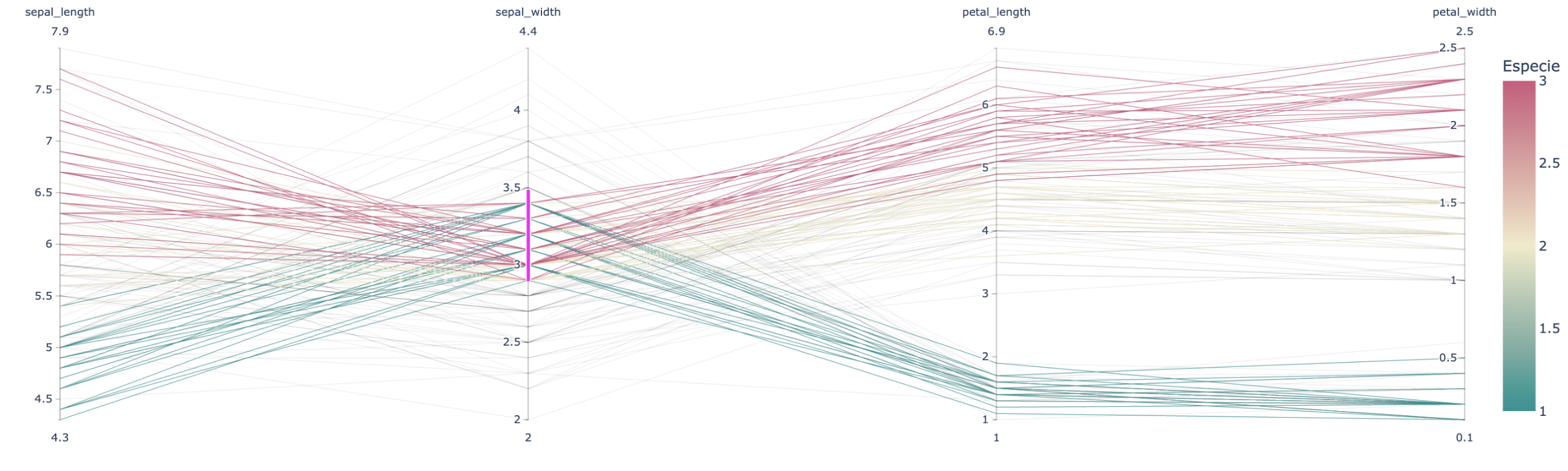
1. Plotly
Maybe probably the most acquainted among the many “lesser-known” choices right here, Plotly has gained traction for its simple method to constructing interactive 2D and 3D visualizations that work in each net and pocket book environments. It helps all kinds of plot sorts—together with some which might be distinctive to Plotly — and could be a superb selection for exhibiting mannequin outcomes, evaluating metrics throughout fashions, and visualizing predictions. Efficiency could be slower with very massive datasets, so profiling is really helpful.
Instance: The parallel coordinates plot represents every function as a parallel vertical axis and reveals how particular person cases transfer throughout options; it might additionally reveal relationships with a goal label.
|
import pandas as pd import plotly.categorical as px
# Iris dataset included in Plotly Specific df = px.knowledge.iris()
# Parallel coordinates plot fig = px.parallel_coordinates( df, dimensions=[‘sepal_length’, ‘sepal_width’, ‘petal_length’, ‘petal_width’], shade=‘species_id’, color_continuous_scale=px.colours.diverging.Tealrose, labels={‘species_id’: ‘Species’}, title=“Plotly-exclusive visualization: Parallel coordinates” ) fig.present() |
Plotly instance
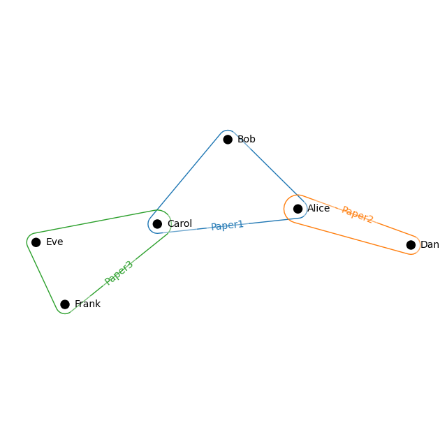
2. HyperNetX
HyperNetX makes a speciality of visualizing hypergraphs — constructions that seize relationships amongst a number of entities (multi-node relationships). Its area of interest is narrower than that of general-purpose plotting libraries, however it may be a compelling choice for sure contexts, significantly when explaining complicated relationships in graphs or in unstructured knowledge reminiscent of textual content.
Instance: A easy hypergraph with multi-node relationships indicating co-authorship of papers (every cyclic edge is a paper) would possibly seem like:
|
pip set up hypernetx networkx |
|
import hypernetx as hnx import networkx as nx
# Instance: small dataset of paper co-authors # Nodes = authors, hyper-edges = papers H = hnx.Hypergraph({ “Paper1”: [“Alice”, “Bob”, “Carol”], “Paper2”: [“Alice”, “Dan”], “Paper3”: [“Carol”, “Eve”, “Frank”] })
hnx.draw(H, with_node_labels=True, with_edge_labels=True) |
HyperNetX instance
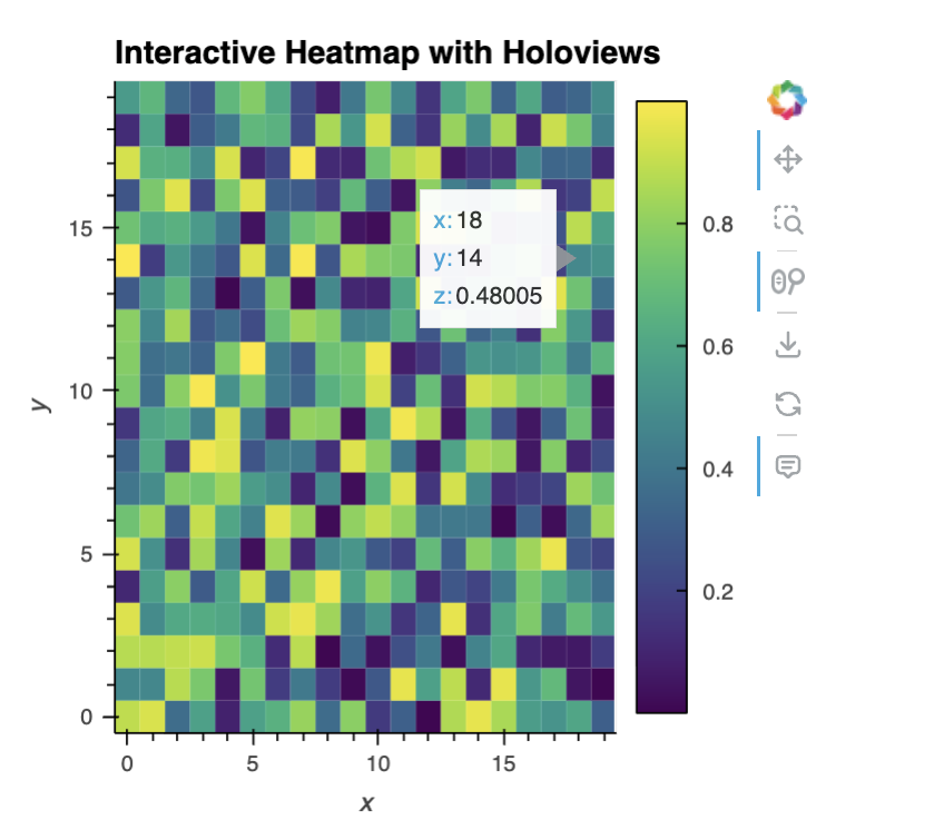
3. HoloViews
HoloViews works with backends reminiscent of Bokeh and Plotly to make declarative, interactive visualizations concise and composable. It’s well-suited for fast exploration with minimal code and could be helpful in machine studying storytelling for exhibiting temporal dynamics, distributional adjustments, and mannequin habits.
Instance: The next snippet shows an interactive heatmap with hover readouts over a 20×20 array of random values, akin to a low-resolution picture.
|
pip set up holoviews bokeh |
|
import holoviews as hv import numpy as np hv.extension(‘bokeh’)
# Instance knowledge: 20 x 20 matrix knowledge = np.random.rand(20, 20)
# Creating an interactive heatmap heatmap = hv.HeatMap([(i, j, data[i,j]) for i in vary(20) for j in vary(20)]) heatmap.opts( width=400, peak=400, instruments=[‘hover’], colorbar=True, cmap=‘Viridis’, title=“Interactive Heatmap with Holoviews” ) |
HoloViews instance
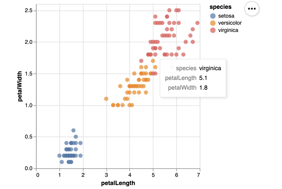
4. Altair
Just like Plotly, Altair affords clear, interactive 2D plots with a chic syntax and first-class export to semi-structured codecs (JSON and Vega) for reuse and downstream formatting. Its 3D assist is proscribed and huge datasets might require downsampling, however it’s a fantastic choice for exploratory storytelling and sharing artifacts in reusable codecs.
Instance: A 2D interactive scatter plot for the Iris dataset utilizing Altair.
|
pip set up altair vega_datasets |
|
import altair as alt from vega_datasets import knowledge
# Iris dataset iris = knowledge.iris()
# Interactive scatter plot: petalLength vs petalWidth, coloured by species chart = alt.Chart(iris).mark_circle(measurement=60).encode( x=‘petalLength’, y=‘petalWidth’, shade=‘species’, tooltip=[‘species’, ‘petalLength’, ‘petalWidth’] ).interactive() # allow zoom and pan
chart |
Altair instance
5. PyDeck
pydeck excels at immersive, interactive 3D visualizations — particularly maps and geospatial knowledge at scale. It’s properly suited to storytelling eventualities reminiscent of plotting ground-truth home costs or mannequin predictions throughout areas (a not-so-subtle nod to a basic public dataset). It’s not meant for easy statistical charts, however loads of different libraries cowl these wants.
Instance: This code builds an aerial, interactive 3D view of the San Francisco space with randomly generated factors rendered as extruded columns at various elevations.
|
1 2 3 4 5 6 7 8 9 10 11 12 13 14 15 16 17 18 19 20 21 22 23 24 25 26 27 28 29 |
import pydeck as pdk import pandas as pd import numpy as np
# Synthetically generated knowledge: 1000 3D factors round San Francisco n = 1000 lat = 37.76 + np.random.randn(n) * 0.01 lon = –122.4 + np.random.randn(n) * 0.01 elev = np.random.rand(n) * 100 # peak for 3D impact knowledge = pd.DataFrame({“lat”: lat, “lon”: lon, “elev”: elev})
# ColumnLayer for extruded columns (helps elevation) layer = pdk.Layer( “ColumnLayer”, knowledge, get_position=‘[lon, lat]’, get_elevation=‘elev’, elevation_scale=1, radius=50, get_fill_color=‘[200, 30, 0, 160]’, pickable=True, )
# Preliminary view view_state = pdk.ViewState(latitude=37.76, longitude=–122.4, zoom=12, pitch=50)
# Full Deck r = pdk.Deck(layers=[layer], initial_view_state=view_state, tooltip={“textual content”: “Elevation: {elev}”}) r.present() |
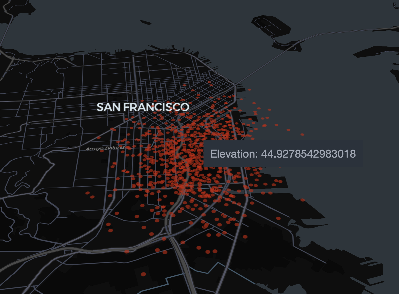
PyDeck instance
Wrapping Up
We explored 5 fascinating, under-the-radar Python visualization libraries and highlighted how their options can improve machine studying storytelling — from hypergraph construction and parallel coordinates to interactive heatmaps, reusable Vega specs, and immersive 3D maps.
5 Lesser-Identified Visualization Libraries for Impactful Machine Studying Storytelling
Picture by Editor | ChatGPT
Introduction
Information storytelling usually extends into machine studying, the place we want partaking visuals that assist a transparent narrative. Whereas standard Python libraries like Matplotlib and its higher-level API, Seaborn, are frequent decisions amongst builders, knowledge scientists, and storytellers alike, there are different libraries value exploring. They provide distinctive options — reminiscent of much less frequent plot sorts and wealthy interactivity — that may strengthen a narrative.
This text briefly presents 5 lesser-known libraries for knowledge visualization that may present added worth in machine studying storytelling, together with brief demonstration examples.
1. Plotly
Maybe probably the most acquainted among the many “lesser-known” choices right here, Plotly has gained traction for its simple method to constructing interactive 2D and 3D visualizations that work in each net and pocket book environments. It helps all kinds of plot sorts—together with some which might be distinctive to Plotly — and could be a superb selection for exhibiting mannequin outcomes, evaluating metrics throughout fashions, and visualizing predictions. Efficiency could be slower with very massive datasets, so profiling is really helpful.
Instance: The parallel coordinates plot represents every function as a parallel vertical axis and reveals how particular person cases transfer throughout options; it might additionally reveal relationships with a goal label.
|
import pandas as pd import plotly.categorical as px
# Iris dataset included in Plotly Specific df = px.knowledge.iris()
# Parallel coordinates plot fig = px.parallel_coordinates( df, dimensions=[‘sepal_length’, ‘sepal_width’, ‘petal_length’, ‘petal_width’], shade=‘species_id’, color_continuous_scale=px.colours.diverging.Tealrose, labels={‘species_id’: ‘Species’}, title=“Plotly-exclusive visualization: Parallel coordinates” ) fig.present() |
Plotly instance
2. HyperNetX
HyperNetX makes a speciality of visualizing hypergraphs — constructions that seize relationships amongst a number of entities (multi-node relationships). Its area of interest is narrower than that of general-purpose plotting libraries, however it may be a compelling choice for sure contexts, significantly when explaining complicated relationships in graphs or in unstructured knowledge reminiscent of textual content.
Instance: A easy hypergraph with multi-node relationships indicating co-authorship of papers (every cyclic edge is a paper) would possibly seem like:
|
pip set up hypernetx networkx |
|
import hypernetx as hnx import networkx as nx
# Instance: small dataset of paper co-authors # Nodes = authors, hyper-edges = papers H = hnx.Hypergraph({ “Paper1”: [“Alice”, “Bob”, “Carol”], “Paper2”: [“Alice”, “Dan”], “Paper3”: [“Carol”, “Eve”, “Frank”] })
hnx.draw(H, with_node_labels=True, with_edge_labels=True) |
HyperNetX instance
3. HoloViews
HoloViews works with backends reminiscent of Bokeh and Plotly to make declarative, interactive visualizations concise and composable. It’s well-suited for fast exploration with minimal code and could be helpful in machine studying storytelling for exhibiting temporal dynamics, distributional adjustments, and mannequin habits.
Instance: The next snippet shows an interactive heatmap with hover readouts over a 20×20 array of random values, akin to a low-resolution picture.
|
pip set up holoviews bokeh |
|
import holoviews as hv import numpy as np hv.extension(‘bokeh’)
# Instance knowledge: 20 x 20 matrix knowledge = np.random.rand(20, 20)
# Creating an interactive heatmap heatmap = hv.HeatMap([(i, j, data[i,j]) for i in vary(20) for j in vary(20)]) heatmap.opts( width=400, peak=400, instruments=[‘hover’], colorbar=True, cmap=‘Viridis’, title=“Interactive Heatmap with Holoviews” ) |
HoloViews instance
4. Altair
Just like Plotly, Altair affords clear, interactive 2D plots with a chic syntax and first-class export to semi-structured codecs (JSON and Vega) for reuse and downstream formatting. Its 3D assist is proscribed and huge datasets might require downsampling, however it’s a fantastic choice for exploratory storytelling and sharing artifacts in reusable codecs.
Instance: A 2D interactive scatter plot for the Iris dataset utilizing Altair.
|
pip set up altair vega_datasets |
|
import altair as alt from vega_datasets import knowledge
# Iris dataset iris = knowledge.iris()
# Interactive scatter plot: petalLength vs petalWidth, coloured by species chart = alt.Chart(iris).mark_circle(measurement=60).encode( x=‘petalLength’, y=‘petalWidth’, shade=‘species’, tooltip=[‘species’, ‘petalLength’, ‘petalWidth’] ).interactive() # allow zoom and pan
chart |
Altair instance
5. PyDeck
pydeck excels at immersive, interactive 3D visualizations — particularly maps and geospatial knowledge at scale. It’s properly suited to storytelling eventualities reminiscent of plotting ground-truth home costs or mannequin predictions throughout areas (a not-so-subtle nod to a basic public dataset). It’s not meant for easy statistical charts, however loads of different libraries cowl these wants.
Instance: This code builds an aerial, interactive 3D view of the San Francisco space with randomly generated factors rendered as extruded columns at various elevations.
|
1 2 3 4 5 6 7 8 9 10 11 12 13 14 15 16 17 18 19 20 21 22 23 24 25 26 27 28 29 |
import pydeck as pdk import pandas as pd import numpy as np
# Synthetically generated knowledge: 1000 3D factors round San Francisco n = 1000 lat = 37.76 + np.random.randn(n) * 0.01 lon = –122.4 + np.random.randn(n) * 0.01 elev = np.random.rand(n) * 100 # peak for 3D impact knowledge = pd.DataFrame({“lat”: lat, “lon”: lon, “elev”: elev})
# ColumnLayer for extruded columns (helps elevation) layer = pdk.Layer( “ColumnLayer”, knowledge, get_position=‘[lon, lat]’, get_elevation=‘elev’, elevation_scale=1, radius=50, get_fill_color=‘[200, 30, 0, 160]’, pickable=True, )
# Preliminary view view_state = pdk.ViewState(latitude=37.76, longitude=–122.4, zoom=12, pitch=50)
# Full Deck r = pdk.Deck(layers=[layer], initial_view_state=view_state, tooltip={“textual content”: “Elevation: {elev}”}) r.present() |
PyDeck instance
Wrapping Up
We explored 5 fascinating, under-the-radar Python visualization libraries and highlighted how their options can improve machine studying storytelling — from hypergraph construction and parallel coordinates to interactive heatmaps, reusable Vega specs, and immersive 3D maps.


